RL for classical feedback control in LIGO
Apply reinforcement learning to design and tune classical feedback controllers that keep LIGO interferometers stably locked.
Research area
LIGO’s mirrors must be held to within $10^{-19}$ meters — roughly one ten-thousandth the diameter of a proton — while remaining free to respond to passing gravitational waves. The feedback controllers that maintain this extraordinary precision also inject noise that masks the very signals LIGO is trying to detect. Below 30 Hz, this control noise — not quantum noise, not seismic noise — is the dominant limit on sensitivity. In collaboration with Google DeepMind and the Gran Sasso Science Institute (GSSI), we developed Deep Loop Shaping (DLS), a reinforcement learning algorithm that designs feedback controllers directly in the frequency domain. Deployed at LIGO Livingston in 2024, DLS reduced control noise by 30–100× across the 10–30 Hz band, expanding LIGO’s reach for observing heavy black hole mergers. The work was published in Science in 2025.
Contents:
- The control challenge
- Classical control design: what humans do
- Deep Loop Shaping: the RL formulation
- From simulation to the real detector
- Results: 30–100× noise reduction
- Competing approaches
- Beyond DARM: other control applications
- Our contributions
- Current status and open questions
- Key references
The control challenge
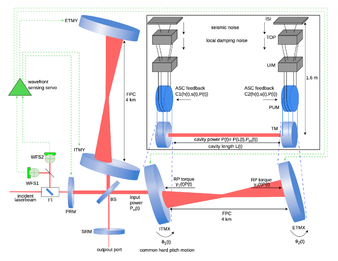
A gravitational-wave interferometer is among the most complex feedback control systems ever built. LIGO must simultaneously regulate dozens of coupled degrees of freedom:
- Length degrees of freedom: DARM (differential arm length — the gravitational-wave signal channel), CARM (common arm length), MICH (Michelson asymmetry), PRCL (power recycling cavity length), SRCL (signal recycling cavity length)
- Angular degrees of freedom: 10 coupled angular DOFs — pitch and yaw for each of 5 suspended optics (two input test masses, two end test masses, beam splitter)
- Auxiliary loops: laser frequency stabilization, intensity stabilization, input mode cleaner, output mode cleaner, squeezer phase locking
Each degree of freedom is controlled through a hierarchy of actuators. The test masses hang as quadruple pendulums — four stages of suspension that provide seismic isolation above ~10 Hz. Actuation forces are applied at different stages depending on the frequency: electromagnetic coil-magnet actuators at the upper stages provide large forces for low-frequency control, while electrostatic drives at the test mass itself provide finer, quieter actuation at higher frequencies.
The plant — the physical system being controlled — is a coupled opto-mechanical system with pendulum dynamics, optical springs from radiation pressure, and cross-couplings between length and angular degrees of freedom. The open-loop transfer function captures this complexity:
\[G_{\text{OL}}(f) = C(f) \cdot P(f)\]| where $C(f)$ is the controller transfer function and $P(f)$ is the plant transfer function. The controller must achieve unity gain — $ | G_{\text{OL}}(f_{\text{UGF}}) | = 1$ — at a carefully chosen frequency (the unity gain frequency, typically 100–200 Hz for DARM), with sufficient phase margin to ensure stability. |
Why pendulums make control hard
A simple pendulum has a transfer function $P(f) \propto 1/(f_0^2 - f^2)$ with a resonance at frequency $f_0$. Above resonance, the response falls as $1/f^2$ — a 180° phase lag. LIGO’s quadruple pendulum has four cascaded stages, giving $1/f^8$ roll-off above ~10 Hz and 720° of accumulated phase lag. The controller must provide enough phase lead to compensate for this lag at the unity gain frequency while maintaining gain margins at all other frequencies. This is fundamentally a frequency-domain design challenge.
Classical control design: what humans do
For the past three decades, LIGO’s feedback controllers have been designed by commissioning scientists using classical frequency-domain techniques: Bode plot shaping, Nyquist stability analysis, and manual pole-zero placement. The process works like this:
-
Measure the plant: Inject broadband excitation signals and measure the transfer function from actuator drive to sensor readout. This gives $P(f)$ — the frequency response of the physical system.
-
Shape the open loop: Design a controller $C(f)$ so that the open-loop transfer function $G_{\text{OL}}(f) = C(f) \cdot P(f)$ has the desired shape: high gain at low frequencies for disturbance rejection, unity gain at the crossover frequency, and sufficient phase margin (typically >30°) and gain margin (typically >6 dB) for robustness.
-
Add notch filters: The mirror suspensions have mechanical resonances (violin modes at ~500 Hz, bounce modes at ~9 Hz) that would destabilize the loop. Narrow notch filters remove these resonances from the open-loop response.
-
Iterate: Adjust the controller, re-measure the closed-loop response, and refine. This process takes weeks to months per degree of freedom.
The fundamental tradeoff that limits this approach is between disturbance rejection and noise injection. The closed-loop control noise spectral density at the detector output is:
\[S_{\text{ctrl}}(f) = \left|\frac{C(f)}{1 + G_{\text{OL}}(f)}\right|^2 S_{\text{act}}(f)\]where $S_{\text{act}}(f)$ is the actuator noise. To suppress seismic disturbances below ~1 Hz, the controller needs high gain at low frequencies — but this gain also amplifies actuator noise, which leaks through the closed-loop transfer function into the gravitational-wave band.
Human designers manage this tradeoff by placing poles and zeros to roll off the controller gain as steeply as possible between the control band and the signal band. But the phase constraints imposed by stability requirements limit how steep this roll-off can be. A human typically places a few integrators and a few roll-off stages — perhaps 10–15 poles and zeros in total. The question is: could a more complex controller, with dozens or hundreds of poles and zeros, thread through the stability constraints more cleverly and achieve a steeper roll-off?
Nyquist stability and why more complex controllers are harder to design by hand
The Nyquist stability criterion states that a closed-loop system is stable if and only if the open-loop transfer function $G_{\text{OL}}(f)$, when plotted in the complex plane as $f$ ranges from 0 to $\infty$, does not encircle the critical point $-1 + 0j$. For a simple controller with few poles and zeros, the Nyquist plot is easy to visualize and reason about. But a controller with many poles and zeros produces a Nyquist plot that weaves through the complex plane in intricate patterns. A human designer cannot easily verify that no part of this complex trajectory comes too close to the critical point. This is why human-designed LIGO controllers tend to be simple — not because simple is optimal, but because simple is verifiable.
The actuator hierarchy: why LIGO uses three stages of actuation
LIGO’s quadruple pendulum suspension provides passive seismic isolation, but the residual motion at the test mass must still be actively controlled. Three actuator stages apply forces at different points on the suspension chain:
| Stage | Actuator type | Force range | Noise floor | Bandwidth |
|---|---|---|---|---|
| Top (M0) | Coil-magnet | Large (~1 mN) | High | DC–10 Hz |
| Penultimate (M2) | Coil-magnet | Medium (~10 μN) | Medium | DC–50 Hz |
| Test mass (M3) | Electrostatic | Small (~1 μN) | Low | DC–1 kHz |
The controller distributes forces across these stages to minimize noise in the GW band: low-frequency forces go to the noisy-but-powerful upper stages, while only the quietest corrections are applied at the test mass. Optimizing this distribution is part of the control design problem.
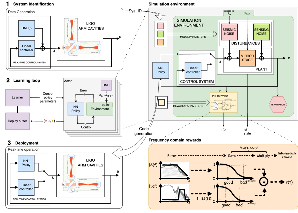
Deep Loop Shaping: the RL formulation
The key insight behind Deep Loop Shaping is that control design specifications are inherently frequency-domain objects — gain margins, phase margins, noise spectral densities, bandwidth requirements. Rather than training an RL agent on time-domain simulations (where it would need millions of steps to discover that a 0.01 Hz oscillation is bad), DLS formulates the problem entirely in the frequency domain.
State: The current controller, represented as a transfer function — a set of poles, zeros, and gain values that define $C(f)$.
Action: Modifications to the controller — adding, removing, or moving poles and zeros, adjusting gains at specific frequency bands.
Reward: A frequency-domain score computed using IIR filter banks. The key innovation is how this score is computed:
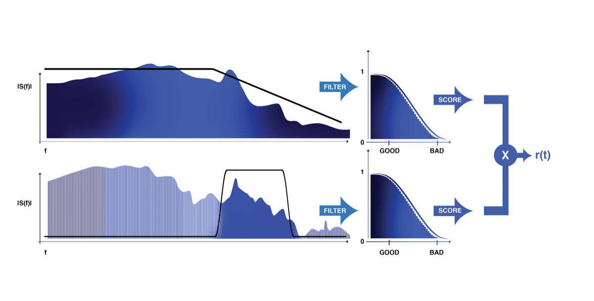
where $F_i(f)$ are IIR filter transfer functions that extract specific frequency-band features, $\sigma$ is the sigmoid function, and the thresholds and scales encode the design specifications (e.g., “the noise spectral density must be below $X$ between 10 and 30 Hz”). The multiplicative structure ensures that the agent cannot trade off one specification against another — every requirement must be met.
The RL algorithm is Maximum a Posteriori Policy Optimization (MPO), a distributed actor-critic method. The agent maintains a policy network that proposes controller modifications and a critic network that estimates expected future reward. Training uses domain randomization — systematic variations in the plant model parameters — to ensure that controllers are robust to modeling errors when deployed on the real detector.
From simulation to the real detector
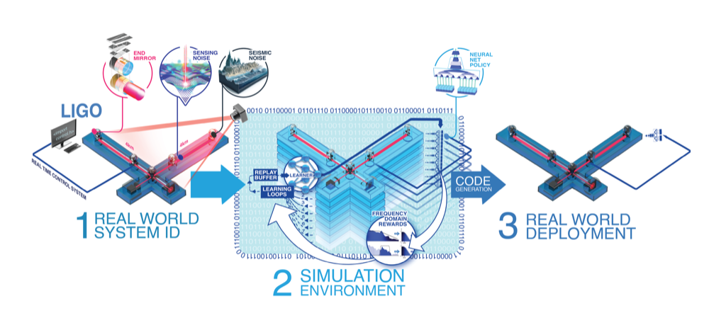
Deploying an RL-designed controller on a $1 billion scientific instrument requires extraordinary care. The DLS pipeline has five stages:
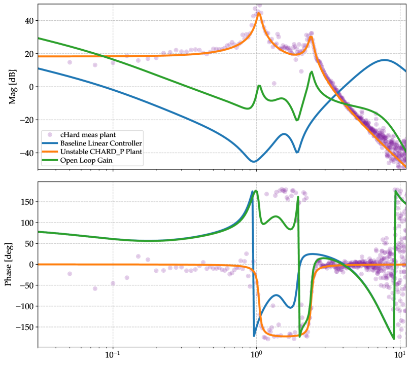
Stage 1: System identification. Broadband excitation signals are injected into the LIGO Livingston (LLO) control system, and the plant transfer function $P(f)$ is measured from the response. This captures the real mechanical, optical, and electronic dynamics of the detector — including nonlinearities and cross-couplings that simple models miss.
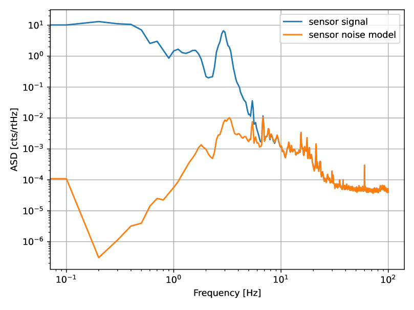
Stage 2: Simulation environment. A faithful simulation of the LIGO control loop is constructed using the measured plant model. This environment includes all the physics that the controller will encounter: pendulum dynamics, optical spring effects, actuator noise models, sensor noise models, and the actuator hierarchy.
Stage 3: RL training. The DLS agent trains in this simulation environment for thousands of iterations, typically completing in hours on a computing cluster. Domain randomization perturbs the plant model during training — varying resonance frequencies, quality factors, and gain calibrations — so the agent learns controllers that are robust to the inevitable mismatch between model and reality.
Stage 4: Candidate validation. Promising controller candidates are tested in progressively more realistic simulations. Stability margins (gain margin, phase margin) are verified across the full range of plant model uncertainties. Only candidates that maintain robust stability under worst-case parameter variations advance to hardware testing.
Stage 5: Hardware deployment. The validated controller is compiled from its neural network representation to ANSI C code for execution on LIGO’s digital control system. The real-time system operates at 16,384 Hz (16 kHz), requiring deterministic execution with bounded latency. The controller is deployed during dedicated commissioning time at LLO, where its performance is compared against the human-designed baseline.
Neural network to real-time C code: how the controller runs at 16 kHz
LIGO’s digital control system is a hard real-time system: every control cycle must complete within 61 μs (1/16384 seconds), with no exceptions. A missed deadline can cause loss of interferometer lock — a catastrophic event that takes hours to recover from. The DLS controller, originally represented as a neural network, is compiled to ANSI C code that implements the equivalent transfer function as a cascade of second-order IIR filter sections (biquads). Each biquad requires only 5 multiplications and 4 additions per sample — well within the computational budget. The total controller typically requires 20–40 biquad sections, consuming less than 1% of the available CPU time on LIGO’s control processors.
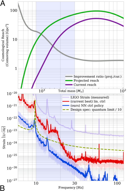
Results: 30–100× noise reduction
Deep Loop Shaping was deployed at LIGO Livingston Observatory in 2024. The results exceeded expectations:
-
Broadband control noise reduction: >30× reduction across the entire 10–30 Hz band — the frequency range critical for observing intermediate-mass black hole (IMBH) mergers and the inspiral phase of heavy stellar-mass binary black holes.
-
Sub-band improvements up to 100×: In specific narrow frequency bands within 10–30 Hz, the DLS controller achieved control noise reductions of up to 100×.
-
Control noise below quantum back-action: For the first time, a classical feedback controller achieved control noise levels below the quantum back-action limit — the noise floor set by the radiation pressure of the laser photons themselves. This means the controller is no longer the limiting noise source at any frequency in the GW band.
-
No stability compromise: The DLS controller maintained gain margins >6 dB and phase margins >30° — matching or exceeding the human-designed baseline. During the one-hour proof-of-concept test at LLO, lock stability was indistinguishable from normal operations.
The improvement translates directly to astrophysical reach. The observable volume for a given source class scales as the cube of the detection distance:
\[\eta = \frac{V_{\text{DLS}}}{V_{\text{baseline}}} = \left(\frac{d_{\text{DLS}}}{d_{\text{baseline}}}\right)^3\]For IMBH mergers ($M \sim 100$–$1000\,M_\odot$), whose gravitational-wave emission peaks in the 10–30 Hz band, the DLS controller significantly expands the cosmological volume accessible to LIGO. The improvement also enables earlier detection of stellar-mass binary mergers during their inspiral phase — giving astronomers more warning time before merger — and improves sensitivity to black holes in eccentric (non-circular) orbits, whose low-frequency gravitational-wave emission was previously buried in control noise.
Competing approaches
Several alternative approaches to feedback controller design exist, each with different strengths and limitations:
Classical PID + notch filters. The current standard at LIGO. Proportional-integral-derivative controllers with hand-placed notch filters for mechanical resonances. Effective and well-understood, but requires expert intuition and does not jointly optimize across frequency bands. The controller complexity is limited by what a human can verify.
$H_\infty$ optimal control. A mathematical framework that minimizes the worst-case gain from disturbances to outputs. Provides formal robustness guarantees and has been applied to gravitational-wave detector control in simulation. However, $H_\infty$ synthesis is conservative by construction — it optimizes for the worst case, which may be overly pessimistic. It also becomes computationally intractable for large MIMO systems.
Adaptive filtering (LMS/RLS). Least-mean-squares and recursive least-squares algorithms for online estimation of optimal filter coefficients. LIGO uses these extensively for feedforward noise subtraction (Wiener filtering of seismic noise, beam jitter noise), but they are designed for feedforward paths, not for feedback loop shaping where stability is a hard constraint.
Kalman filtering. Optimal state estimation given a linear system model and known noise statistics. Used in LIGO for some auxiliary DOF control and for state estimation in lock acquisition. However, Kalman filtering estimates states, not controller shapes — it tells you the best estimate of the mirror position, not the best controller transfer function.
Time-domain RL (PPO, SAC, DDPG). Standard reinforcement learning applied to raw time-series control signals. Proven effective for robotics, drone racing, and game playing. However, for LIGO control, the specifications are frequency-domain objects (noise spectra, stability margins), making time-domain rewards extremely sample-inefficient. An agent would need millions of time-domain steps to evaluate whether a controller injects 1% more noise at 15 Hz.
Generative optical design (Urania). Complementary rather than competing. Urania optimizes the detector topology — which mirrors, beam splitters, and cavities to use and how to connect them. DLS optimizes the controller for a given topology. A combined approach — jointly optimizing topology and controller — is an open research direction.
Beyond DARM: other control applications
The DLS framework was demonstrated on the DARM (differential arm length) degree of freedom — LIGO’s primary gravitational-wave readout channel. But the same approach applies to many other control challenges in gravitational-wave detection:
Lock acquisition. Bringing the interferometer from an uncontrolled state to full resonance is a multi-stage process that currently takes 30 minutes to several hours and frequently fails. Each stage requires a different controller, and the transitions between stages are fragile. RL could optimize the entire lock acquisition sequence — including the transition logic — as a single end-to-end policy.
Angular control. LIGO’s 10 angular degrees of freedom are coupled through radiation pressure torques and misalignment-induced length-to-angle cross-couplings. Currently, each angular loop is designed independently, ignoring cross-couplings. A MIMO extension of DLS could jointly optimize all 10 angular controllers, exploiting the cross-coupling structure rather than fighting it.
Adaptive control. Detector conditions change over time: seismic activity varies with weather and human activity, thermal transients shift optical alignment, and squeezed light injection parameters drift. An adaptive version of DLS could continuously adjust controller parameters in response to changing conditions — maintaining optimal performance without manual intervention.
Auxiliary DOF control. MICH, PRCL, SRCL, and the input mode cleaner all require feedback controllers that inject noise into the gravitational-wave channel through cross-couplings. Optimizing these controllers jointly with DARM could yield additional sensitivity improvements.
Next-generation detectors. Future longer-baseline detectors will have different plant dynamics — longer arms, lower pendulum frequencies, different suspension designs — but the same fundamental control challenges. DLS, being model-based, can be retrained for any plant model, making it directly applicable to next-generation detector design.
Our contributions
-
Improving cosmological reach of a gravitational wave observatory using Deep Loop Shaping — Buchli, Tracey, Andric, Wipf, …, Adhikari, Harms et al., Science, 2025. The DLS algorithm: reinforcement learning with frequency-domain rewards for feedback controller design. First RL-designed controller deployed at a gravitational-wave observatory. Achieved 30–100× control noise reduction at LIGO Livingston, pushing classical control noise below the quantum back-action limit.
-
Noise Reduction in Gravitational-wave Data via Deep Learning — Ormiston, Nguyen, Coughlin, Adhikari & Katsavounidis, Physical Review Research, 2020. DeepClean: a convolutional neural network for post-hoc noise subtraction from LIGO data. Demonstrated that machine learning could improve LIGO sensitivity by identifying and removing nonlinear noise couplings — an early proof of concept that preceded and motivated the DLS work.
-
Digital Discovery of Interferometric Gravitational Wave Detectors — Krenn, Drori & Adhikari, Physical Review X, 2025. The Urania algorithm and the GW Detector Zoo: complementary AI work that optimizes detector topology rather than the controller. The detector topologies discovered by Urania will need controllers designed by DLS or its successors.
-
Nonlinear Noise Cleaning in GW Detectors with CNNs — Yu & Adhikari, Frontiers in AI, 2022. Demonstrated CNN-based noise cleaning that captures nonlinear couplings missed by linear Wiener filters — part of the group’s broader program of applying AI to gravitational-wave instrumentation.
Current status and open questions
Deep Loop Shaping has demonstrated that reinforcement learning can design controllers for one of the most demanding control problems in physics. Several open research directions remain:
Sim-to-real robustness. The current DLS pipeline uses domain randomization to bridge the gap between the simulation model and the real detector. How much randomization is needed? Can formal robustness certificates (e.g., from robust control theory) be combined with RL training to provide stronger guarantees?
Online adaptation. DLS currently trains offline: the agent learns in simulation, and the resulting controller is deployed as a static transfer function. Could the agent adapt in real time during observation runs — continuously adjusting the controller as detector conditions change? This would require safety guarantees that the adaptation cannot destabilize the interferometer.
MIMO extension. The Science 2025 result is SISO: DLS optimizes a single-input single-output controller for the DARM loop. Extending to full MIMO — jointly optimizing all length and angular controllers — is the natural next step. The challenge is that the MIMO design space is vastly larger, and stability constraints become more complex (the Nyquist criterion generalizes to the multivariable Nyquist criterion involving the spectral radius of the return ratio matrix).
Integration with Urania. Currently, DLS optimizes the controller for a given detector topology, and Urania optimizes the topology assuming a standard controller. Co-optimizing both simultaneously — where the RL agent can modify both the optical layout and the feedback controller — could discover configurations that neither approach finds alone.
Scaling to next-generation detectors. Future detectors with longer arms, silicon test masses at cryogenic temperatures, and fundamentally different suspension dynamics will pose new challenges. Can DLS controllers trained on LIGO models transfer to these new instruments, or will entirely new training be required? Understanding the generalization properties of RL-designed controllers across detector generations is an open question.
Key references
The DLS paper
- Buchli, Tracey, Andric, Wipf, …, Adhikari, Harms et al. “Improving cosmological reach of a gravitational wave observatory using Deep Loop Shaping.” Science (2025). DOI: 10.1126/science.adw1291 — The primary reference: RL-designed feedback controller deployed at LIGO Livingston, 30–100× control noise reduction, first demonstration that RL can surpass human experts in GW detector control design.
Classical control foundations
-
Åström & Murray. Feedback Systems: An Introduction for Scientists and Engineers. Princeton University Press (2008). — Standard reference for classical and modern control theory, including Bode, Nyquist, and root-locus methods.
-
Skogestad & Postlethwaite. Multivariable Feedback Control: Analysis and Design. Wiley (2005). — Comprehensive treatment of MIMO control, $H_\infty$ synthesis, and robustness analysis.
-
Bode, H.W. Network Analysis and Feedback Amplifier Design. Van Nostrand (1945). — The foundational work on frequency-domain feedback design; established the gain-phase relationships that constrain all feedback controllers.
-
Nyquist, H. “Regeneration theory.” Bell System Technical Journal 11, 126 (1932). — The stability criterion: a feedback system is stable iff the open-loop transfer function does not encircle −1 in the complex plane.
LIGO control systems
-
Staley, Martynov, Abbott et al. “Achieving resonance in the Advanced LIGO gravitational-wave interferometer.” Classical and Quantum Gravity 31, 245010 (2014). — Lock acquisition: the multi-stage process of bringing Advanced LIGO from uncontrolled to fully resonant.
-
LIGO Scientific Collaboration (Aasi, Abbott, Adhikari et al.) “Advanced LIGO.” Classical and Quantum Gravity 32, 074001 (2015). — The Advanced LIGO design paper, including the feedback control architecture for all length and angular degrees of freedom.
-
Buikema, Cahillane, Mansell et al. “Sensitivity and performance of the Advanced LIGO detectors in the third observing run.” Physical Review D 102, 062003 (2020). — O3 detector performance, including control noise contributions to the overall noise budget.
Reinforcement learning foundations
-
Schulman, Wolski, Dhariwal et al. “Proximal Policy Optimization algorithms.” arXiv:1707.06347 (2017). — PPO: the workhorse on-policy RL algorithm. DLS uses MPO instead, but PPO established the paradigm of clipped surrogate objectives for stable policy gradient training.
-
Abdolmaleki, Springenberg, Tassa et al. “Maximum a Posteriori Policy Optimisation.” ICLR (2018). — MPO: the off-policy actor-critic algorithm used by DLS. Combines maximum a posteriori estimation with distributional policy updates.
-
Lillicrap, Hunt, Pritzel et al. “Continuous control with deep reinforcement learning.” ICLR (2016). — DDPG: deep deterministic policy gradient, foundational continuous-action RL method.
RL for real-world control
-
Hwangbo, Lee, Dosovitskiy et al. “Learning agile and dynamic motor skills for legged robots.” Science Robotics 4 (2019). — RL for quadruped locomotion: demonstrated sim-to-real transfer for complex physical systems, inspiring the DLS approach.
-
Kaufmann, Bauersfeld, Loquercio et al. “Champion-level drone racing using deep reinforcement learning.” Nature 620, 982 (2023). — RL exceeding human expert performance in physical control — a direct analogy to DLS surpassing human-designed LIGO controllers.
Complementary AI work at EGG
-
Ormiston, Nguyen, Coughlin, Adhikari & Katsavounidis. “Noise Reduction in Gravitational-wave Data via Deep Learning.” Physical Review Research 2, 033066 (2020). DOI: 10.1103/physrevresearch.2.033066 — DeepClean: neural network noise subtraction from recorded GW data.
-
Yu & Adhikari. “Nonlinear Noise Cleaning in Gravitational-Wave Detectors with Convolutional Neural Networks.” Frontiers in AI 5, 811563 (2022). DOI: 10.3389/frai.2022.811563 — CNN for nonlinear noise coupling removal.
-
Yu, Adhikari, Magee, Sachdev & Chen. “Early warning of coalescing neutron-star and neutron-star-black-hole binaries from the nonstationary noise background using neural networks.” Physical Review D 104, 062004 (2021). DOI: 10.1103/physrevd.104.062004 — Neural networks for low-latency GW event detection.
-
Krenn, Drori & Adhikari. “Digital Discovery of Interferometric Gravitational Wave Detectors.” Physical Review X 15, 021012 (2025). DOI: 10.1103/physrevx.15.021012 — Urania: computational discovery of novel detector topologies.
Detector science targets
-
Adhikari, Arai, Brooks, Wipf et al. “A cryogenic silicon interferometer for gravitational-wave detection.” Classical and Quantum Gravity 37, 165003 (2020). — LIGO Voyager design and noise budget, including control noise as a limiting noise source below 30 Hz.
-
Mandel & Farmer. “Merging stellar-mass binary black holes.” Physics Reports 955, 1 (2022). — Science case for observing intermediate-mass and heavy stellar-mass black hole mergers in the 10–100 Hz band — the frequency range where DLS has the greatest impact.
-
Evans, Adhikari, Afle et al. “A Horizon Study for Cosmic Explorer.” arXiv:2109.09882 (2021). — Science targets and control system challenges for next-generation detectors.