Quantum Neural Networks for Optimal Coherent Control

Gravitational-wave detectors operate near the standard quantum limit — but “near” is not “at.” The gap between achieved sensitivity and fundamental quantum bounds is, at its core, a control problem: how to prepare the optimal quantum state of light entering the interferometer, and how to extract the maximum information from the light leaving it. Classical feedback controllers, no matter how sophisticated, cannot close this gap because they destroy quantum correlations the moment they make a measurement. Coherent quantum control — where quantum systems control other quantum systems without collapsing their states — offers a path beyond this barrier.

Quantum neural networks (QNNs) bring the optimization power of machine learning to this problem. Rather than hand-designing control strategies from first principles, QNNs learn optimal coherent transformations directly — discovering measurement bases and control protocols that approach fundamental quantum bounds.

Contents:

• What is coherent quantum control?
• The information-theoretic view
• QNN architectures for quantum control
• Optimal measurement strategies
• Scaling relations and performance bounds
• Connection to non-Gaussian states
• Connection to PSOMA
• Competing approaches
• Implementation challenges
• Connections to other fields
• Our contributions
• Current status and future directions
• Key references
• Further reading

What is coherent quantum control?

Classical feedback: measure, then act

In classical feedback control — the backbone of every operating GW detector — a sensor measures the system, a computer processes the measurement, and an actuator corrects the system. This works beautifully for classical disturbances: seismic noise, thermal drifts, angular misalignments. But it has a fundamental limitation: measurement destroys quantum information.

When a homodyne detector measures the amplitude quadrature of light, it irreversibly projects out the phase quadrature. Any quantum correlations between the two — precisely the correlations that squeezing creates — are lost. The measurement record is classical; all subsequent processing, no matter how clever, operates on this classical record.

Coherent feedback: quantum systems controlling quantum systems

Coherent feedback replaces the classical measurement with a quantum interaction. Instead of measuring the output field and feeding back a classical signal, a coherent controller couples directly to the quantum field — reflecting it off an auxiliary cavity, passing it through a nonlinear crystal, or routing it through a photonic circuit — without ever collapsing the quantum state.

The Wiseman-Milburn framework (1993, 1994) formalized this distinction. They showed that for certain control objectives — particularly those involving quantum noise reduction — coherent feedback can outperform any measurement-based strategy. The intuition: a coherent controller can process both quadratures simultaneously, preserving quantum correlations that measurement-based feedback necessarily destroys.

This is where QNNs enter: they provide a systematic framework for discovering optimal coherent controllers — parameterized quantum circuits whose parameters are optimized to minimize a cost function (e.g., estimation variance, state preparation fidelity, or detection SNR).

The information-theoretic view

Quantum Fisher information

The quantum Cramér-Rao bound (QCRB) sets the ultimate precision with which a parameter $\theta$ can be estimated from a quantum state $\rho(\theta)$:

where $\nu$ is the number of independent measurements and $F_Q$ is the quantum Fisher information (QFI):

The multiparameter problem

A single gravitational-wave event carries information about multiple parameters: chirp mass $\mathcal{M}$, mass ratio $q$, spins $\chi_1, \chi_2$, luminosity distance $d_L$, sky position $(\theta, \phi)$, inclination $\iota$, and polarization $\psi$. Each parameter is encoded in different features of the signal — amplitude, phase, frequency evolution, polarization content.

For a single parameter, homodyne detection can saturate the QCRB by choosing the right measurement quadrature. But for multiple parameters simultaneously, no single quadrature is optimal for all — this is the incompatibility of quantum measurements for non-commuting observables. The multiparameter QCRB involves the quantum Fisher information matrix:

and the achievable precision is bounded by:

The gap between what homodyne detection achieves and what the multiparameter QCRB permits is the information loss — and it’s this gap that QNNs aim to close.

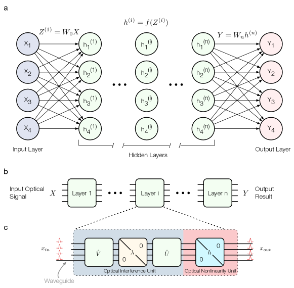
QNN architectures for quantum control

Photonic neural networks

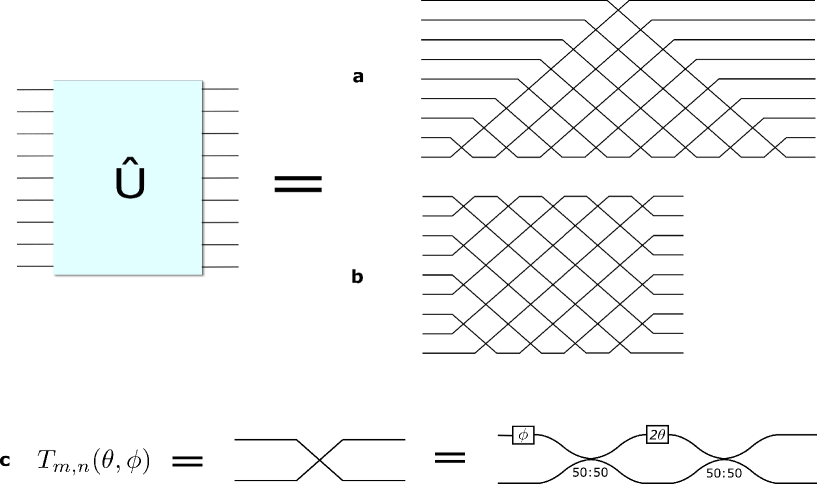
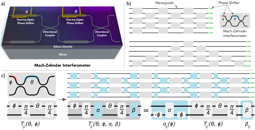
The most mature QNN architecture for optical systems: programmable meshes of Mach-Zehnder interferometers (MZIs) that implement arbitrary unitary transformations on $N$ optical modes. Reck et al. (1994) showed that any $N \times N$ unitary can be decomposed into $N(N-1)/2$ beamsplitters and $N$ phase shifters. Clements et al. (2016) improved this to a more hardware-efficient rectangular mesh.

Each MZI has two tunable parameters (internal and external phase shifts). For an $N$-mode network, the full parameterization has $N^2$ degrees of freedom — enough to implement any unitary in $U(N)$. Training proceeds by gradient descent on a classical computer, computing the gradient of a cost function with respect to all phase parameters, then updating the physical phase shifters.

For GW readout: A photonic neural network placed after the interferometer output port would transform the $N$ spatial/temporal modes of the output field before they reach the photodetectors. By optimizing the transformation, the network learns to project onto the measurement basis that maximizes Fisher information for a target set of source parameters.

Experimental demonstrations: Shen et al. (2017) built a 4-layer photonic neural network with 56 MZIs for vowel recognition. Carolan et al. (2015) demonstrated a 6-mode universal photonic processor. Harris et al. (2018) showed a programmable 8×8 mesh operating at GHz bandwidth.

Variational quantum circuits

Parameterized quantum circuits — alternating layers of entangling gates and single-mode rotations — that can approximate arbitrary quantum channels. Unlike photonic meshes (which implement only unitaries), variational circuits can include non-unitary operations (measurement, conditional preparation) and classical feedback within the circuit.

The circuit is described by a parameter vector $\boldsymbol{\theta} = (\theta_1, \ldots, \theta_p)$, and the cost function $C(\boldsymbol{\theta})$ is minimized by a classical optimizer. Gradients can be computed via the parameter-shift rule:

This requires only two circuit evaluations per parameter — no backpropagation through quantum hardware.

Killoran et al. (2019) extended variational circuits to continuous-variable (CV) systems — precisely the domain of quantum optics. Their CV-QNN uses layers of interferometers, squeezers, displacements, and Kerr nonlinearities as trainable gates. Applied to GW parameter estimation, a CV-QNN can learn measurement strategies that approach the multiparameter QCRB on simulated data.

Tensor network classifiers

Matrix product states (MPS) and tree tensor networks provide efficient classical representations of quantum states with bounded entanglement. As classifiers, they naturally capture correlations at multiple scales — ideal for time-frequency data like GW spectrograms.

Stoudenmire & Schwab (2016) showed that MPS classifiers match or exceed CNNs on image recognition benchmarks while requiring fewer parameters and providing interpretable representations. For GW data analysis, tensor network classifiers offer a principled bridge between quantum information structure and signal processing.

Optimal measurement strategies

Why homodyne is suboptimal

Balanced homodyne detection measures one quadrature of the electromagnetic field:

where $\phi$ is the local oscillator phase. For a single parameter encoded in a known quadrature, this is optimal. But for multiparameter estimation — or when the signal quadrature varies with frequency — homodyne discards information in the orthogonal quadrature.

Frequency-dependent squeezing (now operational in LIGO) rotates the squeezed quadrature as a function of frequency using a 300-meter filter cavity. This optimizes the input state, but the readout remains fixed homodyne. The two optimizations — input state and measurement basis — are coupled, and jointly optimizing both is where QNNs provide their advantage.

Adaptive measurement

Rather than choosing a fixed measurement basis, an adaptive protocol adjusts the measurement on each shot based on previous outcomes. Wiseman (1995) showed that adaptive homodyne — where the local oscillator phase is updated in real time based on the photocurrent — can saturate the QCRB for phase estimation with coherent states. Berry & Wiseman (2000) extended this to squeezed states.

For transient GW signals (compact binary mergers), the signal-to-noise ratio accumulates over time. An adaptive QNN could update its measurement basis as the signal sweeps through the detector band, progressively narrowing the parameter estimates. This is the quantum analog of matched filtering — but operating on the quantum field rather than a classical data stream.

Photon-counting and hybrid readout

Photon-number-resolving (PNR) detection accesses information that homodyne detection cannot — it directly measures the photon statistics of the field. For non-Gaussian states (cat states, GKP states, Fock states), PNR detection can extract Fisher information that homodyne necessarily misses.

A QNN can learn to route different frequency bands to different detector types — homodyne for bands where squeezing is dominant, photon counting for bands where non-Gaussian features are important — implementing a hybrid readout that outperforms either alone.

Scaling relations and performance bounds

The quantum metrology hierarchy

Multi-mode scaling

A GW detector’s output field has many modes — continuous in frequency, with quantum correlations (from squeezing) coupling different frequency bins. An $N$-mode QNN processing the output can, in principle, capture correlations across $N$ frequency bins. The Fisher information accessible to the QNN scales as:

where $C_{jk}$ are quantum cross-correlations between modes $j$ and $k$. Squeezed light creates non-zero $C_{jk}$; a QNN that exploits these correlations can extract more information than independent single-mode homodyne.

Connection to non-Gaussian states

The QNN and non-Gaussian state projects are two sides of the same optimization: what is the best quantum state to inject into the interferometer, and what is the best measurement to perform on the output?

For Gaussian states (coherent + squeezed), homodyne detection is close to optimal — the QNN adds modest improvement through multiparameter optimization. But for non-Gaussian states, the advantage of QNN-optimized readout becomes dramatic:

• Cat states carry phase information in their interference fringes — homodyne averages over these fringes, losing most of the Fisher information. A QNN-optimized photon-counting scheme can access it.
• GKP states encode information in a lattice structure in phase space — extracting this requires modular measurements that homodyne cannot implement.
• Photon-subtracted squeezed states have non-Gaussian Wigner functions — their Fisher information advantage over squeezed states is only realized with non-Gaussian detection.

A QNN framework treats state preparation and readout as a joint optimization problem: given a fixed loss budget and available nonlinear resources, what is the globally optimal input state + measurement combination? This is a variational problem over the space of quantum channels — exactly what variational quantum circuits are designed to solve.

Connection to PSOMA

The Phase-Sensitive Optomechanical Amplifier (PSOMA) changes the optimal control strategy in a fundamental way. PSOMA uses radiation-pressure coupling between the GW signal and an auxiliary mechanical oscillator to achieve phase-sensitive amplification — boosting the signal quadrature while squeezing the noise quadrature.

When PSOMA operates before the readout:

• The signal-to-noise ratio is enhanced in a frequency band around the mechanical resonance
• The quantum correlations in the output field are modified — creating frequency-dependent entanglement between signal and idler modes
• The optimal measurement basis shifts: instead of homodyne at a fixed angle, the optimal readout must account for the frequency-dependent squeezing angle imposed by PSOMA

A QNN trained on the PSOMA output field can learn to exploit these modified correlations. Crucially, PSOMA + QNN is not simply “amplify then measure” — the QNN can co-optimize with the PSOMA parameters (detuning, coupling strength) to find operating points where the combination outperforms either alone.

Competing approaches

Classical optimal control

Model-based classical controllers (LQG, $\mathcal{H}_\infty$, Kalman filtering) are the current standard for GW detector control. They excel when the system model is known and the noise is Gaussian. Limitations:

• They operate on classical measurement records — quantum information is already lost
• They require an accurate system model — model mismatch degrades performance
• They cannot exploit quantum correlations between the controlled system and the controller

Reinforcement learning for quantum systems

Classical RL agents interacting with quantum systems via measurements. The Deep Loop Shaping project in our group applies this to LIGO’s classical control loops. For quantum control, RL has been used to discover pulse sequences for quantum state preparation (Bukov et al. 2018) and to optimize measurement protocols (Fösel et al. 2018).

Key distinction: RL controllers make classical decisions based on measurement outcomes. QNNs implement coherent quantum operations that preserve quantum information. RL is optimal for classical control tasks; QNNs address the regime where quantum coherence matters.

Model-based quantum control (GRAPE, Krotov)

Gradient-based optimization of quantum control pulses — the “model-based” counterpart to QNNs. GRAPE (Gradient Ascent Pulse Engineering, Khaneja et al. 2005) and Krotov’s method compute exact gradients through the quantum dynamics. These are powerful when the system Hamiltonian is known precisely.

What QNNs add: Model-free optimization. When the system model is imperfect — as it inevitably is for a complex detector with $10^5$ degrees of freedom — QNNs can learn directly from experimental data, adapting to the actual system rather than a model of it. The parameter-shift rule enables gradient computation on quantum hardware without requiring a system model.

Direct measurement optimization

Designing optimal POVMs (positive operator-valued measures) analytically for specific estimation problems. For single-parameter estimation with known signal model, this is often tractable and gives the best possible measurement. For multiparameter estimation with uncertain signal models — the GW detection scenario — the POVM space is too large for analytical optimization, and QNNs provide a practical search strategy.

Implementation challenges

Wavelength compatibility

Current photonic neural networks operate at telecom wavelengths (1550 nm) on silicon photonic chips. GW detectors operate at 1064 nm (current LIGO) or ~2 µm (Voyager). Adapting photonic processors to these wavelengths requires:

• 1064 nm: Lithium niobate or silicon nitride platforms (both demonstrated but less mature than silicon photonics)
• 2 µm: Chalcogenide or germanium-on-silicon platforms (early stage)

Alternatively, the SFG project could convert the 2 µm output to ~700 nm, where silicon photonics operates natively — potentially enabling QNN processing at the converted wavelength.

Training on quantum hardware

QNNs cannot be trained with standard backpropagation — the quantum operations are not classically differentiable in the usual sense. Practical training approaches:

• Parameter-shift rule: Compute gradients by evaluating the circuit at shifted parameters. Requires $2p$ circuit evaluations for $p$ parameters — feasible for circuits with <1000 parameters.
• Quantum natural gradient: Accounts for the Riemannian geometry of quantum state space, leading to faster convergence. Requires estimating the quantum Fisher information matrix at each step — expensive but provably optimal.
• Classical pre-training: Train on a classical simulation of the quantum system, then fine-tune on quantum hardware. This “transfer learning” approach reduces the number of expensive quantum evaluations.

Decoherence during processing

Any QNN processing the interferometer output must operate faster than the decoherence time of the relevant quantum correlations. For audio-frequency squeezing, the relevant timescale is set by the squeezing bandwidth (~100 Hz for current filter cavities, corresponding to ~10 ms). A photonic QNN operating at GHz clock rates has $\sim 10^7$ operations within this window — more than sufficient.

Scalability

Current photonic processors handle 8–12 modes. A GW detector’s output has effectively infinite modes (continuous frequency spectrum). Practical approaches to this mismatch:

• Temporal mode decomposition: Decompose the output into a finite set of temporal modes (pulse shapes) that capture most of the signal information
• Frequency binning: Digitize the spectrum into $N$ bins and process with an $N$-mode QNN
• Hierarchical processing: Cascade multiple small QNNs, each handling a subset of modes, with classical coordination between stages

Connections to other fields

Our contributions

These publications establish the theoretical and experimental foundations for QNN-optimized quantum control in gravitational-wave detectors:

• Displacement noise-free interferometers (Gefen, Tarafder, Adhikari & Chen 2024) — Established quantum precision limits for interferometer topologies that cancel displacement noise, showing how measurement strategy determines the achievable quantum advantage.

• Broadband quantum enhancement (Ganapathy et al. 2023) — Demonstrated frequency-dependent squeezing in LIGO, achieving broadband quantum enhancement of a GW detector — the baseline that QNN-optimized readout aims to surpass.

• Fundamental quantum limit (Miao, Adhikari, et al. 2017) — Established the fundamental quantum limit for linear measurements of classical forces, defining the theoretical ceiling that coherent quantum control approaches.

• PSOMA (Bai, Venugopalan, …, Chen & Adhikari 2020) — Proposed the phase-sensitive optomechanical amplifier as a new quantum control element for GW detectors, whose output statistics are a natural target for QNN-optimized readout.

• Deep learning for GW detectors (Buchli, Tracey, Wipf, Adhikari, et al. 2025) — Demonstrated that deep reinforcement learning can design feedback controllers that improve real LIGO detector performance — establishing the classical-control baseline for quantum extensions.

• Nonlinear noise cleaning (Yu & Adhikari 2022) — Showed that neural networks can learn nonlinear noise couplings in GW detectors, providing a classical preprocessing step that improves the quantum signal-to-noise ratio available to downstream QNN processing.

Current status and future directions

Current status: The QNN project is in the theoretical development and simulation phase. We are:

• Modeling multiparameter estimation performance for different QNN architectures on simulated LIGO output states
• Quantifying the information gap between homodyne readout and the multiparameter QCRB for realistic GW signals
• Evaluating CV-QNN architectures (Killoran et al.) for continuous-variable quantum control relevant to interferometric readout

Near-term goals:

• Quantify the achievable Fisher information gain from QNN-optimized readout vs. fixed homodyne for realistic binary merger parameter estimation
• Design a tabletop proof-of-principle experiment: a small photonic QNN processing the output of a Mach-Zehnder interferometer with squeezed light input
• Develop training protocols that work with limited quantum data (few-shot learning, classical pre-training + quantum fine-tuning)

Open questions:

• Practical advantage threshold: How many photonic modes does a QNN need to outperform optimized homodyne? The answer determines hardware requirements.
• Barren plateaus: Large variational quantum circuits can have exponentially vanishing gradients (“barren plateaus”), making training intractable. Does the structure of quantum metrology cost functions avoid this problem?
• Noise resilience: Photonic circuits have ~0.1 dB loss per MZI. For a 12-mode network (~66 MZIs), total loss is ~6.6 dB. At what point does QNN processing loss outweigh the information gain?
• Integration architecture: Where in the LIGO readout chain does a QNN provide the most benefit — after the output Faraday isolator, after the output mode cleaner, or integrated into the squeezing injection path?

Key references

Coherent quantum control theory

• Wiseman & Milburn, “Quantum theory of optical feedback via homodyne detection,” PRL 70, 548 (1993). DOI:10.1103/PhysRevLett.70.548 — Founded the theory of measurement-based quantum feedback.
• Wiseman & Milburn, “All-optical versus electro-optical quantum-limited feedback,” PRA 49, 4110 (1994). DOI:10.1103/PhysRevA.49.4110 — Proved coherent feedback can outperform measurement-based feedback.
• Lloyd, “Coherent quantum feedback,” PRA 62, 022108 (2000). DOI:10.1103/PhysRevA.62.022108 — General framework for coherent feedback networks.
• Nurdin, James & Doherty, “Network synthesis of linear dynamical quantum stochastic systems,” SIAM J. Control Optim. 48, 2686 (2009). DOI:10.1137/080728652 — Systematic design of coherent feedback networks.

Photonic neural networks

• Reck et al., “Experimental realization of any discrete unitary operator,” PRL 73, 58 (1994). DOI:10.1103/PhysRevLett.73.58 — Proved any unitary can be decomposed into beamsplitters and phase shifters.
• Clements et al., “Optimal design for universal multiport interferometers,” Optica 3, 1460 (2016). DOI:10.1364/OPTICA.3.001460 — Hardware-efficient rectangular mesh design.
• Shen et al., “Deep learning with coherent nanophotonic circuits,” Nat. Photonics 11, 441 (2017). DOI:10.1038/nphoton.2017.93 — Experimental photonic neural network.
• Harris et al., “Linear programmable nanophotonic processors,” Nat. Photonics 12, 1 (2018). DOI:10.1038/s41566-018-0232-2 — Programmable 8×8 photonic mesh at GHz speed.

Variational quantum circuits and CV-QNN

• Killoran et al., “Continuous-variable quantum neural networks,” PRA 99, 032338 (2019). DOI:10.1103/PhysRevA.99.032338 — CV-QNN architecture for quantum optics.
• Cerezo et al., “Variational quantum algorithms,” Nat. Rev. Phys. 3, 625 (2021). DOI:10.1038/s42254-021-00348-9 — Comprehensive review of variational quantum methods.
• Schuld et al., “Evaluating analytic gradients on quantum hardware,” PRA 99, 032331 (2019). DOI:10.1103/PhysRevA.99.032331 — The parameter-shift rule for quantum gradient computation.

Quantum metrology theory

• Braunstein & Caves, “Statistical distance and the geometry of quantum states,” PRL 72, 3439 (1994). DOI:10.1103/PhysRevLett.72.3439 — Quantum Fisher information and the QCRB.
• Giovannetti, Lloyd & Maccone, “Quantum metrology,” PRL 96, 010401 (2006). DOI:10.1103/PhysRevLett.96.010401 — Heisenberg limit for quantum-enhanced metrology.
• Demkowicz-Dobrzański, Jarzyna & Kołodyński, “Quantum limits in optical interferometry,” Prog. Optics 60, 345 (2015). DOI:10.1016/bs.po.2015.02.003 — Comprehensive review of quantum limits with loss.

Adaptive quantum measurement

• Wiseman, “Adaptive phase measurements of optical modes,” PRL 75, 4587 (1995). DOI:10.1103/PhysRevLett.75.4587 — Adaptive homodyne saturates the QCRB.
• Berry & Wiseman, “Optimal states and almost optimal adaptive measurements for quantum interferometry,” PRL 85, 5098 (2000). DOI:10.1103/PhysRevLett.85.5098 — Adaptive measurement with squeezed states.

Tensor networks for classification

• Stoudenmire & Schwab, “Supervised learning with tensor networks,” NeurIPS (2016). arXiv:1605.05775 — MPS classifiers matching CNN performance.

Further reading

• Wiseman & Milburn, Quantum Measurement and Control (Cambridge, 2009) — The standard textbook on quantum feedback, measurement theory, and quantum control.
• Weedbrook et al., “Gaussian quantum information,” Rev. Mod. Phys. 84, 621 (2012). DOI:10.1103/RevModPhys.84.621 — Comprehensive review of Gaussian quantum information — the foundation on which non-Gaussian and QNN approaches build.
• Tóth & Apellaniz, “Quantum metrology from a quantum information science perspective,” J. Phys. A 47, 424006 (2014). DOI:10.1088/1751-8113/47/42/424006 — Connecting quantum metrology to quantum information.
• Steinbrecher et al., “Quantum optical neural networks,” npj Quantum Inf. 5, 60 (2019). DOI:10.1038/s41534-019-0174-7 — Quantum optical neural networks with experimental demonstrations.