Neural Network Noise Cleaning

Below ~60 Hz, LIGO’s sensitivity is limited not by fundamental quantum noise but by control noise — auxiliary feedback loops that keep the interferometer locked inadvertently inject disturbances into the gravitational-wave readout. These couplings are often nonlinear and non-stationary, making them invisible to traditional linear subtraction techniques like Wiener filtering. We use neural networks to learn and remove these noise sources directly from detector data — a post-hoc approach that cleans recorded strain data, complementing the real-time controller design pursued in RL Feedback Control.

Contents:

• The noise subtraction problem
• DeepClean: learning nonlinear couplings
• Physics-informed CNN architecture
• The bilinear coupling model
• Early warning for compact binary mergers
• Why neural networks? Competing approaches
• Signal safety and validation
• Connections to other EGG projects
• Our contributions
• Current status and open questions
• Key references
• Further reading

---

The noise subtraction problem

Witness channels and the subtraction concept

LIGO has thousands of auxiliary sensor channels — accelerometers, magnetometers, optical lever sensors, beam spot monitors, and control signal readouts — that witness environmental and instrumental disturbances. If the coupling between a witness channel $w(t)$ and the gravitational-wave strain $h(t)$ is known, the noise contribution can be subtracted:

\[h_\text{clean}(t) = h(t) - \hat{n}(t; w_1, w_2, \ldots, w_N)\]

where $\hat{n}(t)$ is the noise estimate constructed from $N$ witness channels. The challenge is building $\hat{n}$ accurately. A Wiener filter assumes the coupling is linear and stationary:

\[\hat{n}_\text{Wiener}(t) = \sum_i \int g_i(\tau)\, w_i(t - \tau)\, d\tau\]

where each $g_i(\tau)$ is a time-invariant transfer function. This works well for some noise sources — for example, subtracting 60 Hz power-line harmonics that couple linearly through electromagnetic pickup. But the dominant noise below 60 Hz is neither linear nor stationary.

Why linear methods fail

The primary source of excess noise below 60 Hz is angular control. LIGO’s test masses must be aligned to microradians to maintain the optical cavity resonance. The alignment system uses optical levers (OPLEVs) and wavefront sensors to measure angular misalignment and applies corrective torques through electromagnetic actuators. These feedback loops keep the beam centered, but they inject noise into the gravitational-wave channel through two mechanisms:

1. Direct actuation noise: Electronic noise in the angular control servos drives the test masses, creating differential arm-length fluctuations.
2. Beam-spot coupling: When the laser beam hits the test mass off-center, angular motion of the mirror couples into apparent length change. The coupling strength is proportional to the beam-spot offset — a quantity that drifts on timescales of minutes to hours.

The second mechanism is the killer: it creates a bilinear coupling where a slowly drifting parameter (beam-spot position) modulates a fast oscillatory signal (angular control noise). Wiener filters, which assume time-invariant linear transfer functions, cannot capture this.

The coherence clue: why auxiliary channels carry the information

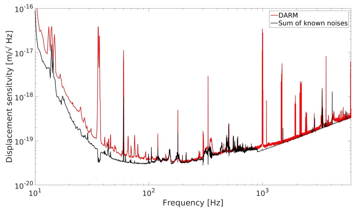
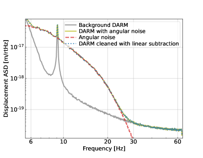
The key diagnostic is the coherence between auxiliary channels and DARM (the gravitational-wave readout). If a witness channel $w(t)$ is coherent with DARM at some frequency $f$, it means $w(t)$ carries information about the noise at that frequency — and subtraction is possible.

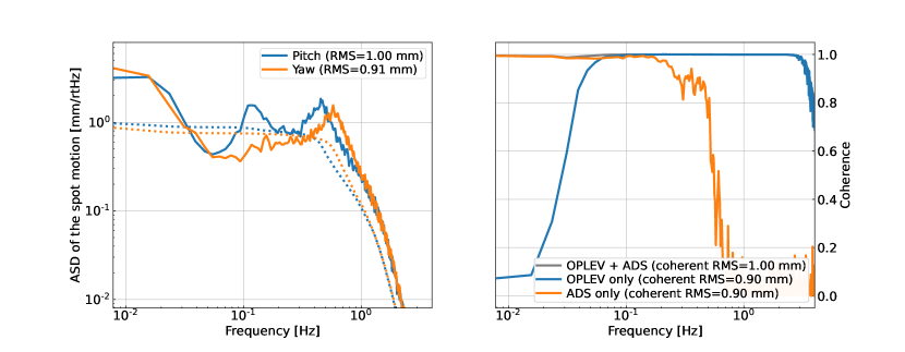
For angular noise, the OPLEV and angular drive signals (ADS) show high coherence with DARM below ~1 Hz. But the coherence drops above ~1 Hz because the coupling becomes nonlinear: the beam-spot position (measured by OPLEVs) modulates the angular control signal (measured by ADS). No single linear channel captures the full coupling. A nonlinear model that multiplies OPLEV and ADS signals can recover the lost coherence.

This is precisely what the “slow $\times$ fast” CNN architecture exploits — it learns the multiplication that the physics demands.

---

DeepClean: learning nonlinear couplings

DeepClean (Ormiston, Nguyen, Coughlin, Adhikari & Katsavounidis, 2020) is our foundational framework for neural network noise subtraction. It trains a deep neural network to map auxiliary sensor channels directly to the noise they inject into the gravitational-wave readout — learning whatever coupling function the data demands, without assuming linearity or stationarity.

Architecture and training

The DeepClean pipeline has three stages:

1. Preprocessing: Witness channels and strain data are bandpass-filtered and downsampled to the frequency range of interest (~10–60 Hz). The strain channel is used as the training target.
2. Training: A convolutional neural network processes time-series segments from multiple witness channels simultaneously, predicting the noise contribution $\hat{n}(t)$. The loss function combines a time-domain mean-squared-error term with a frequency-domain PSD term that directly penalizes excess noise power in the target band.
3. Inference: The trained network predicts $\hat{n}(t)$ on new data, which is subtracted from the strain: $h_\text{clean}(t) = h(t) - \hat{n}(t)$.

Results: outperforming Wiener filters

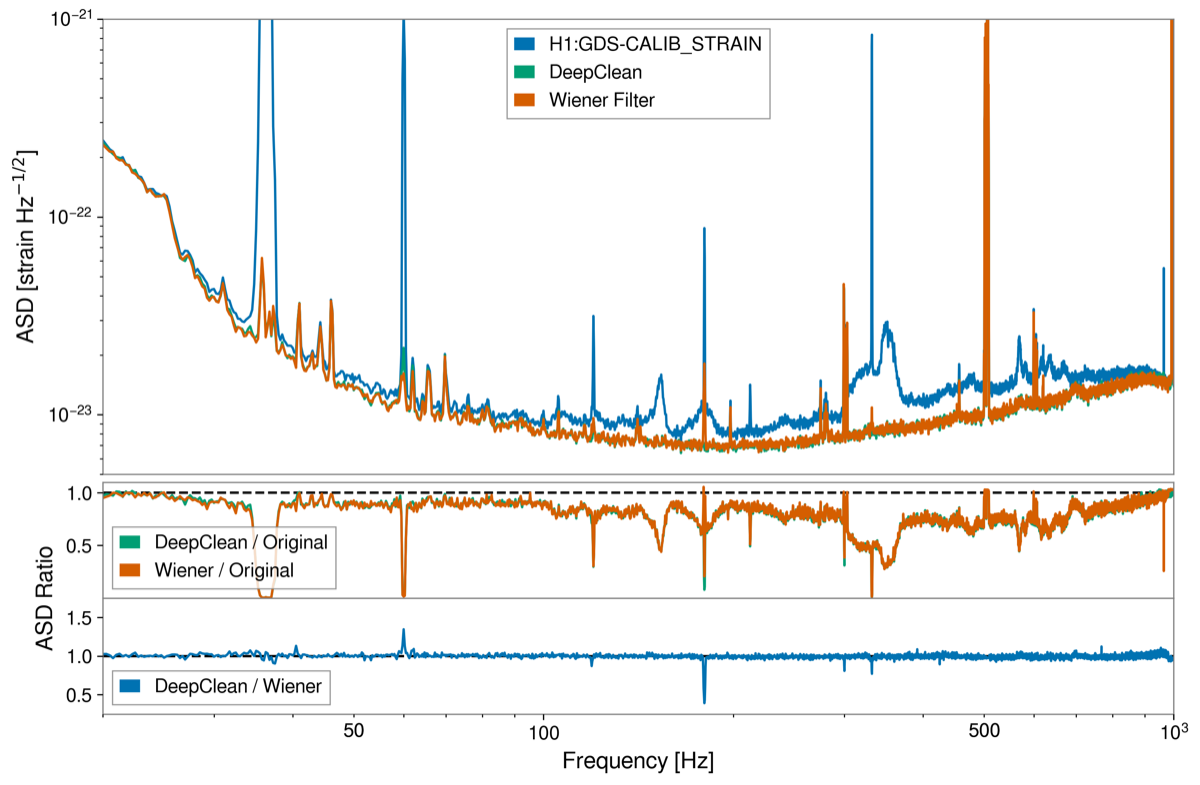
Applied to LIGO Hanford data from the second observing run (O2), DeepClean achieves:

• ~22% improvement in signal-to-noise ratio for detected binary black hole mergers
• Noise reduction across the 20–100 Hz band, with particularly strong subtraction of spectral lines and broadband excess
• Consistent parameter estimation: posterior distributions for source masses, spins, and distance remain unchanged after cleaning — the signal is preserved while noise is removed

How DeepClean preserves gravitational-wave signals

A critical concern with any noise subtraction method is signal safety: could the network accidentally learn to subtract part of the gravitational-wave signal along with the noise? DeepClean protects against this through two mechanisms:

Architecture-level protection: The network takes only auxiliary witness channels as input — never the strain channel itself. Since gravitational waves do not appear in auxiliary sensors (they are decoupled from the differential arm length at the sensitivity level of auxiliary instruments), the network has no information about the signal content and cannot subtract it.

Empirical validation: Ormiston et al. performed parameter estimation on binary black hole events before and after DeepClean subtraction. The posterior distributions for component masses, effective spin, luminosity distance, and sky location were statistically consistent — confirming that the cleaning process does not bias astrophysical inference.

This architectural separation between witness channels and strain is the key design principle. The neural network is a sophisticated noise estimator, but it can only estimate noise from what it sees — and it never sees the gravitational-wave signal.

---

Physics-informed CNN architecture

While DeepClean demonstrated that neural networks can outperform Wiener filters, it used a generic CNN architecture that treated all input channels uniformly. Building on this, Yu & Adhikari (2022) developed a physics-informed CNN that encodes the known structure of the dominant coupling mechanism directly into the network architecture.

The slow-times-fast decomposition

The key physics insight is that angular control noise couples to DARM through a bilinear mechanism: slow beam-spot drifts (timescale: minutes to hours) modulate fast angular control signals (timescale: milliseconds). Mathematically, the noise contribution takes the form:

\[n(t) \approx x_\text{spot}(t) \times \theta_\text{ctrl}(t)\]

where $x_\text{spot}(t)$ is the beam-spot position on the test mass (a slowly varying quantity) and $\theta_\text{ctrl}(t)$ is the angular control signal (a fast oscillatory signal). This product of slow and fast time series cannot be captured by any linear filter.

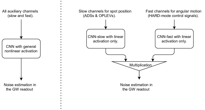
The physics-informed architecture splits the CNN into two branches:

Branch	Input channels	Timescale	Activation
CNN-slow	OPLEVs, beam spot monitors (ADS)	0.01–1 Hz	Linear only
CNN-fast	HARD-mode angular control signals	1–60 Hz	Linear only

Each branch uses linear activations only — no ReLU, no sigmoid. The outputs of the two branches are then multiplied element-wise to produce the noise estimate. This multiplication is the only nonlinearity in the network, and it directly encodes the bilinear coupling that the physics predicts.

Why linear branches with a multiplicative junction?

The choice to restrict each branch to linear activations may seem surprising — why remove the neural network’s ability to learn arbitrary nonlinearities? The answer lies in the structure of the problem.

The bilinear coupling $n \propto x_\text{spot} \times \theta_\text{ctrl}$ means that the noise is linear in $x_\text{spot}$ for fixed $\theta_\text{ctrl}$, and linear in $\theta_\text{ctrl}$ for fixed $x_\text{spot}$. The only nonlinearity is their product. By enforcing linearity within each branch, the architecture constrains the network to learn exactly this structure — preventing overfitting to noise or accidental subtraction of the gravitational-wave signal.

A generic CNN with nonlinear activations has far more expressive power, but that extra capacity is a liability: it can fit noise in the training data and generalize poorly to new data. The physics-informed architecture trades off expressiveness for robustness and interpretability.

This is a concrete example of the general principle that encoding known physics into machine learning architectures — rather than relying on the network to discover it from data — leads to better generalization with less training data.

Curriculum learning for non-stationary noise

The beam-spot position drifts over time, so the coupling strength is non-stationary. Yu & Adhikari introduced a curriculum learning strategy to handle this:

1. Stage 1: Train on data segments where the beam-spot drift is small (quasi-stationary regime). The network learns the basic coupling structure.
2. Stage 2: Gradually include data segments with larger drifts, increasing the non-stationarity. The network learns to track the slowly evolving coupling.

This staged approach converges faster and to lower residual noise than training on all data simultaneously — the network first masters the easy cases, then progressively handles harder ones.

Performance comparison

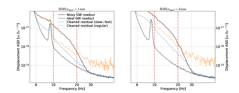
The slow-times-fast architecture demonstrates clear advantages:

• At 1 mm RMS beam-spot drift: both architectures perform comparably, with the slow-times-fast having a slight edge below 15 Hz
• At 3 mm RMS beam-spot drift: the slow-times-fast architecture significantly outperforms the generic CNN, especially in the 10–30 Hz band where the bilinear coupling dominates
• The residual after slow-times-fast cleaning approaches the ideal noise-free readout — the physics-based constraint extracts nearly all the nonlinear noise

---

The bilinear coupling model

Physical origin

The fundamental mechanism is length-to-angle coupling in a Fabry-Perot cavity. When a laser beam hits a mirror off-center by a distance $\delta x$, a mirror tilt $\delta\theta$ produces an apparent cavity length change:

\[\delta L \approx \delta x \times \delta\theta\]

In LIGO, the beam-spot position $\delta x$ drifts on slow timescales due to thermal effects, seismic settling, and alignment control offsets. The angular motion $\delta\theta$ oscillates at the frequencies of the angular control loops (up to tens of Hz). Their product creates noise in the gravitational-wave readout at frequencies set by the angular control bandwidth — precisely the 10–60 Hz band where LIGO’s sensitivity needs the most improvement.

Quantitative coupling estimate

For a Fabry-Perot arm cavity of length $L = 4$ km with finesse $\mathcal{F} \approx 450$:

• Beam-spot offset: $\delta x \sim 1$ mm (typical RMS during O3)
• Angular control noise: $\delta\theta \sim 10^{-8}$ rad/$\sqrt{\text{Hz}}$ at 20 Hz
• Length noise: $\delta L = \delta x \times \delta\theta \sim 10^{-11}$ m/$\sqrt{\text{Hz}}$
• Strain noise: $\delta L / L \sim 2.5 \times 10^{-15}$ Hz$^{-1/2}$ at 20 Hz

This is comparable to the measured excess noise in LIGO below 30 Hz, confirming that angular-to-length bilinear coupling is a (if not the) dominant noise source in this band.

The coupling is bilinear because the beam-spot offset is an effectively DC quantity (it drifts on minute timescales) that multiplies the AC angular noise. At any instant, the coupling appears linear — but the linear transfer function changes as the beam spot drifts. A Wiener filter fit at one time becomes stale minutes later.

Why this coupling is hard to model analytically

In principle, if we knew $\delta x(t)$ and $\delta\theta(t)$ perfectly, we could compute and subtract $\delta L(t) = \delta x(t) \times \delta\theta(t)$ without any machine learning. In practice:

• Multiple coupling paths: There are four test masses, each with pitch and yaw degrees of freedom, plus coupling from the beam splitter and recycling mirrors — dozens of bilinear coupling paths that must be subtracted simultaneously.
• Higher-order couplings: The simple $\delta x \times \delta\theta$ model is the leading-order term. Higher-order couplings (e.g., spot size variations, cavity mode distortions) add additional nonlinear terms.
• Calibration uncertainty: The transfer functions from witness channels to the actual beam-spot offset and angular motion have frequency-dependent calibration errors that propagate into the subtraction.
• Non-stationarity: The coupling drifts not only because the beam spot moves, but because the angular control loop gains change (due to optical power variations, alignment drifts, and commissioning adjustments).

A neural network bypasses all of these complications by learning the end-to-end mapping from witness channels to noise — whatever the coupling actually is, not what we think it should be.

---

Early warning for compact binary mergers

The same noise-cleaning framework enables a qualitatively new capability: pre-merger early warning of compact binary coalescences.

The science case

A binary neutron star (BNS) inspiral sweeps upward in frequency — it enters LIGO’s sensitive band minutes before merger. At the current sensitivity floor of ~20 Hz, a typical BNS spends only ~100 seconds in band before merger. But if the low-frequency noise floor could be pushed down to ~10 Hz, the same signal would be visible for ~1000 seconds — nearly 17 minutes before merger.

This extra lead time is transformative for multi-messenger astronomy: electromagnetic telescopes (optical, X-ray, gamma-ray, radio) need tens of seconds to slew to the source location. With conventional pipelines operating on uncleaned data, the warning time for a BNS at 40 Mpc is typically only a few seconds — not enough for telescope response.

Neural network early warning

Yu, Adhikari, Magee, Sachdev & Chen (2021) demonstrated that combining neural network noise cleaning with matched-filter detection creates a compound neural network system for early warning:

1. Stage 1 — Noise cleaning: A CNN (using the slow-times-fast architecture) subtracts control noise from the strain data in the 10–30 Hz band.
2. Stage 2 — Detection: A matched-filter search runs on the cleaned data, achieving sensitivity at lower frequencies than is possible on raw data.

Why early warning requires noise cleaning

The frequency of a BNS inspiral signal at time $\tau$ before merger is approximately:

\[f(\tau) \approx 134 \;\text{Hz}\;\left(\frac{1.2\,M_\odot}{\mathcal{M}_c}\right)^{5/8} \left(\frac{1\;\text{s}}{\tau}\right)^{3/8}\]

where $\mathcal{M}c$ is the chirp mass. For a typical BNS with $\mathcal{M}_c \approx 1.2\,M\odot$:

Time before merger $\tau$	Frequency $f$
1000 s (~17 min)	~10 Hz
100 s	~24 Hz
10 s	~56 Hz
1 s	~134 Hz

The signal spends most of its time below 30 Hz — precisely the band where control noise dominates. Without noise cleaning, matched filters cannot accumulate SNR at these frequencies, and the signal remains buried until it sweeps through the cleaner 30–100 Hz band in the final seconds. Neural network noise cleaning unlocks the low-frequency band, allowing detection minutes earlier.

The SNR accumulation argument

The matched-filter signal-to-noise ratio accumulates as:

\[\rho^2 = 4 \int_{f_\text{low}}^{f_\text{high}} \frac{|\tilde{h}(f)|^2}{S_n(f)}\, df\]

where $\tilde{h}(f)$ is the signal Fourier transform and $S_n(f)$ is the one-sided noise power spectral density. For a BNS inspiral, $

\tilde{h}(f)

^2 \propto f^{-7/3}$ — the signal power is concentrated at low frequencies.

If $S_n(f)$ is dominated by control noise below 30 Hz (say, 10$\times$ above the fundamental noise floor), then reducing $S_n(f)$ by a factor of 10 through neural network cleaning increases the integrand by 10$\times$ in that band. Since the signal itself is strongest at low frequencies ($f^{-7/3}$ weighting), the SNR improvement from cleaning the 10–30 Hz band is disproportionately large.

Yu et al. showed that this SNR improvement translates directly into earlier detection: the matched filter crosses the detection threshold at a lower instantaneous frequency, which corresponds to an earlier time before merger.

---

Why neural networks? Competing approaches

Neural networks are not the only approach to noise subtraction in gravitational-wave detectors. Here we compare the leading alternatives and explain why neural networks offer the best combination of capability and practicality for the nonlinear, non-stationary noise sources that dominate below 60 Hz.

Wiener filtering

The traditional workhorse of noise subtraction. Wiener filters find the optimal linear transfer function between witness channels and the target noise. They are fast to compute, well-understood theoretically, and provably optimal for linear-stationary coupling.

Limitation: Cannot capture bilinear or higher-order couplings. For angular control noise — the dominant source below 60 Hz — Wiener filters leave significant residual noise (as shown in the DeepClean comparison above).

Bilinear subtraction (analytical)

Explicitly multiply pairs of witness channels to create new “virtual” channels, then apply Wiener filtering to the augmented channel set. This directly targets the $x_\text{spot} \times \theta_\text{ctrl}$ coupling.

Limitation: Requires knowing which channel pairs to multiply — a combinatorial problem with thousands of auxiliary channels. Also fails for higher-order couplings and for coupling paths that are not purely bilinear.

Non-parametric regression (kernel methods, Gaussian processes)

Gaussian process regression can model nonlinear functions without specifying the functional form. Applied to noise subtraction, a GP could learn the mapping from witness channels to noise without assuming linearity.

Limitation: Computational cost scales as $\mathcal{O}(N^3)$ with the number of training samples $N$. LIGO data at 16384 Hz produces millions of samples per hour — far beyond the practical limit of GP regression. Sparse approximations help but sacrifice the very flexibility that motivates the non-parametric approach.

Dictionary learning / sparse coding

Represent the noise as a sparse linear combination of basis functions learned from data. The basis can capture some non-stationarity through time-varying coefficients.

Limitation: Still fundamentally linear in the basis functions. Capturing bilinear coupling requires pre-computing cross-product basis elements, returning to the combinatorial problem.

Neural networks: the best fit for this problem

Neural networks combine three properties that match the noise subtraction problem:

1. Nonlinear function approximation: Universal approximation guarantees that sufficiently large networks can model any continuous mapping from witness channels to noise.
2. Scalability: Inference is fast — milliseconds per segment — enabling processing of the entire LIGO data stream.
3. Architecture flexibility: Physics can be encoded directly into the network structure (as in the slow-times-fast architecture), constraining the model where we have knowledge while leaving flexibility where we don’t.

The practical limitation is generalization: a network trained on one observing run may not transfer to the next, because the detector hardware and coupling mechanisms change. This motivates ongoing work on transfer learning and adaptive training strategies.

---

Signal safety and validation

Any noise subtraction technique applied to gravitational-wave data must satisfy a stringent requirement: the astrophysical signal must not be distorted. If the cleaning process removes or distorts even a fraction of a percent of the signal, it corrupts the parameter estimation that determines source masses, spins, distances, and sky locations.

Architectural safeguards

The primary protection is input isolation: the neural network receives only auxiliary witness channels as input, never the gravitational-wave strain itself. Since gravitational waves couple to the differential arm length but not to auxiliary sensors (beam spot monitors, optical levers, magnetometers), the network has no mechanism to learn the signal.

Empirical validation

Ormiston et al. validated signal preservation by performing full Bayesian parameter estimation on binary black hole events before and after DeepClean processing. The posterior distributions for all physical parameters — component masses, effective spin $\chi_\text{eff}$, luminosity distance, and sky location — were statistically consistent, with no evidence of bias.

Hardware injection tests

LIGO routinely injects simulated gravitational-wave signals into the detector hardware by driving the test masses with known waveforms. These injections provide end-to-end validation: if the neural network preserves injected signals with known parameters, it can be trusted on real signals.

---

Connections to other EGG projects

---

Our contributions

• DeepClean (Ormiston, Nguyen, Coughlin, Adhikari & Katsavounidis, 2020) — Introduced deep learning for gravitational-wave noise subtraction. Demonstrated that neural networks outperform Wiener filters for nonlinear noise coupling, achieving ~22% SNR improvement for binary black hole mergers. Established the hybrid PSD + MSE loss function and the principle of witness-only input for signal safety.

• Physics-informed CNN for nonlinear noise cleaning (Yu & Adhikari, 2022) — Developed the “slow $\times$ fast” CNN architecture that encodes the bilinear coupling mechanism directly into the network structure. Demonstrated superior performance over generic CNNs, especially for large beam-spot drifts. Introduced curriculum learning for non-stationary noise.

• Neural network early warning (Yu, Adhikari, Magee, Sachdev & Chen, 2021) — Showed that neural network noise cleaning enables pre-merger early warning for binary neutron star coalescences, providing hundreds of seconds of warning at 40 Mpc and tens of seconds at 160 Mpc — a qualitatively new capability for multi-messenger astronomy.

---

Current status and open questions

Current status: Neural network noise subtraction has been demonstrated on LIGO O2 and O3 data in offline analysis, with validated signal preservation for compact binary merger signals. The physics-informed slow-times-fast architecture has been shown to outperform generic networks on simulated non-stationary data. Early warning capability has been demonstrated in simulation.

Open questions

• Real-time deployment: DeepClean and its successors currently run on recorded data. Deploying neural network noise subtraction in real time — with latency low enough for early-warning alerts — requires inference times under ~100 ms on streaming data. What hardware (GPUs, TPUs, FPGAs) and software architectures make this feasible? Can the slow-times-fast architecture, with its linear branches and single multiplicative junction, be implemented efficiently on low-latency hardware?

• Transfer learning across observing runs: Noise couplings change between observing runs as hardware is modified and the detector is recommissioned. How quickly can models be retrained or adapted when the detector configuration changes? Can features learned in one observing run transfer to the next, reducing the need for full retraining? The physics-informed architecture may have an advantage here: the slow-times-fast structure is valid across runs (the bilinear coupling mechanism persists), even if the specific transfer functions change.

• Deeper into the noise floor: Below ~30 Hz, after control noise is subtracted, what noise sources remain dominant? Newtonian noise from seismic density fluctuations, scattered light, and suspension thermal noise each have different coupling mechanisms. Can neural networks learn to subtract these as well, or do they require different approaches? Newtonian noise, in particular, has a fundamentally different character — it is not an instrumental artifact but a real gravitational signal from the local environment.

• Validation at scale: Gravitational-wave catalogs now contain hundreds of events. Demonstrating signal preservation event-by-event is necessary but not sufficient — systematic biases that are small for individual events could accumulate across a population. Can neural network cleaning be validated at the population level?

• Integration with low-latency pipelines: The early warning application requires not just fast inference but integration with existing LIGO/Virgo/KAGRA low-latency pipelines (GstLAL, PyCBC Live, SPIIR). What interface and data format standards are needed? How should the cleaning uncertainty be propagated into detection significance and sky localization?

---

Key references

EGG publications

• Ormiston, Nguyen, Coughlin, Adhikari & Katsavounidis, “Noise Reduction in Gravitational-wave Data via Deep Learning,” Phys. Rev. Research 2, 033066 (2020). DOI:10.1103/PhysRevResearch.2.033066 — The DeepClean framework: neural network noise subtraction outperforming Wiener filters.

• Yu & Adhikari, “Nonlinear Noise Cleaning in Gravitational-Wave Detectors With Convolutional Neural Networks,” Front. Artif. Intell. 5, 811563 (2022). DOI:10.3389/frai.2022.811563 — Physics-informed slow-times-fast CNN architecture for bilinear noise coupling.

• Yu, Adhikari, Magee, Sachdev & Chen, “Early warning of coalescing neutron-star and neutron-star-black-hole binaries from the nonstationary noise background using neural networks,” Phys. Rev. D 104, 062004 (2021). DOI:10.1103/PhysRevD.104.062004 — Neural network cleaning enables pre-merger early warning for multi-messenger astronomy.

Noise subtraction foundations

• Allen, “Wiener filtering with a seismic array for gravitational wave interferometer noise subtraction,” Phys. Rev. D 60, 029901 (1999). DOI:10.1103/PhysRevD.60.029901 — Foundational paper on Wiener filter noise subtraction for GW detectors.

• Davis et al., “Utilizing aLIGO Glitch Classifications to Validate Gravitational-Wave Candidates,” CQG 38, 135014 (2021). DOI:10.1088/1361-6382/abfd85 — Data quality and glitch classification context for noise subtraction.

• Driggers et al., “Improving astrophysical parameter estimation via offline noise subtraction for Advanced LIGO,” Phys. Rev. D 99, 042001 (2019). DOI:10.1103/PhysRevD.99.042001 — Linear noise subtraction applied to LIGO O2 data, establishing the baseline that DeepClean improves upon.

Machine learning for gravitational waves

• George & Huerta, “Deep Learning for real-time gravitational wave detection and parameter estimation: Results with Advanced LIGO data,” Phys. Lett. B 778, 64 (2018). DOI:10.1016/j.physletb.2017.12.053 — Early demonstration of deep learning for GW signal detection.

• Gabbard et al., “Matching Matched Filtering with Deep Networks for Gravitational-Wave Astronomy,” PRL 120, 141103 (2018). DOI:10.1103/PhysRevLett.120.141103 — CNNs approaching matched-filter sensitivity for BBH detection.

• Cuoco et al., “Enhancing Gravitational-Wave Science with Machine Learning,” Machine Learning: Science and Technology 2, 011002 (2021). DOI:10.1088/2632-2153/abb93a — Comprehensive review of ML applications in GW physics.

LIGO noise characterization

• Buikema et al., “Sensitivity and performance of the Advanced LIGO detectors in the third observing run,” Phys. Rev. D 102, 062003 (2020). DOI:10.1103/PhysRevD.102.062003 — O3 detector performance and noise budget.

• Aasi et al., “Advanced LIGO,” CQG 32, 074001 (2015). DOI:10.1088/0264-9381/32/7/074001 — Advanced LIGO instrument paper.

Related detector noise subtraction

• Vajente et al., “Machine-learning nonstationary noise out of gravitational-wave detectors,” Phys. Rev. D 101, 042003 (2020). DOI:10.1103/PhysRevD.101.042003 — Independent ML approach to non-stationary noise subtraction.

• Mogushi, “Reduction of transient noise artifacts in gravitational-wave data using deep learning,” Phys. Rev. D 104, 124033 (2021). DOI:10.1103/PhysRevD.104.124033 — Neural network removal of transient glitches (complementary to broadband noise cleaning).

• Soni et al., “Discovering features in gravitational-wave data through detector characterization, citizen science and machine learning,” CQG 38, 195016 (2021). DOI:10.1088/1361-6382/ac1ccb — Integrating ML with traditional detector characterization.

---

Further reading

For readers who want to go deeper:

• Goodfellow, Bengio & Courville, Deep Learning (MIT Press, 2016) — Standard textbook covering CNNs, training dynamics, and regularization. Chapters 9–11 are most relevant for understanding the architectures used in DeepClean.

• Saulson, Fundamentals of Interferometric Gravitational Wave Detectors, 2nd ed. (World Scientific, 2017) — Comprehensive treatment of LIGO noise sources, including the control system noise that neural network cleaning targets.

• Fritschel, “Second generation instruments for the Laser Interferometer Gravitational Wave Observatory (LIGO),” Proc. SPIE 4856, 282 (2003). DOI:10.1117/12.459079 — Technical overview of Advanced LIGO control systems and noise couplings.

• Mukund et al., “Transient classification in LIGO data using difference boosting neural network,” Phys. Rev. D 95, 104059 (2017). DOI:10.1103/PhysRevD.95.104059 — Early application of neural networks to LIGO data quality.