Digital-Twin Diagnostics & Forecasting

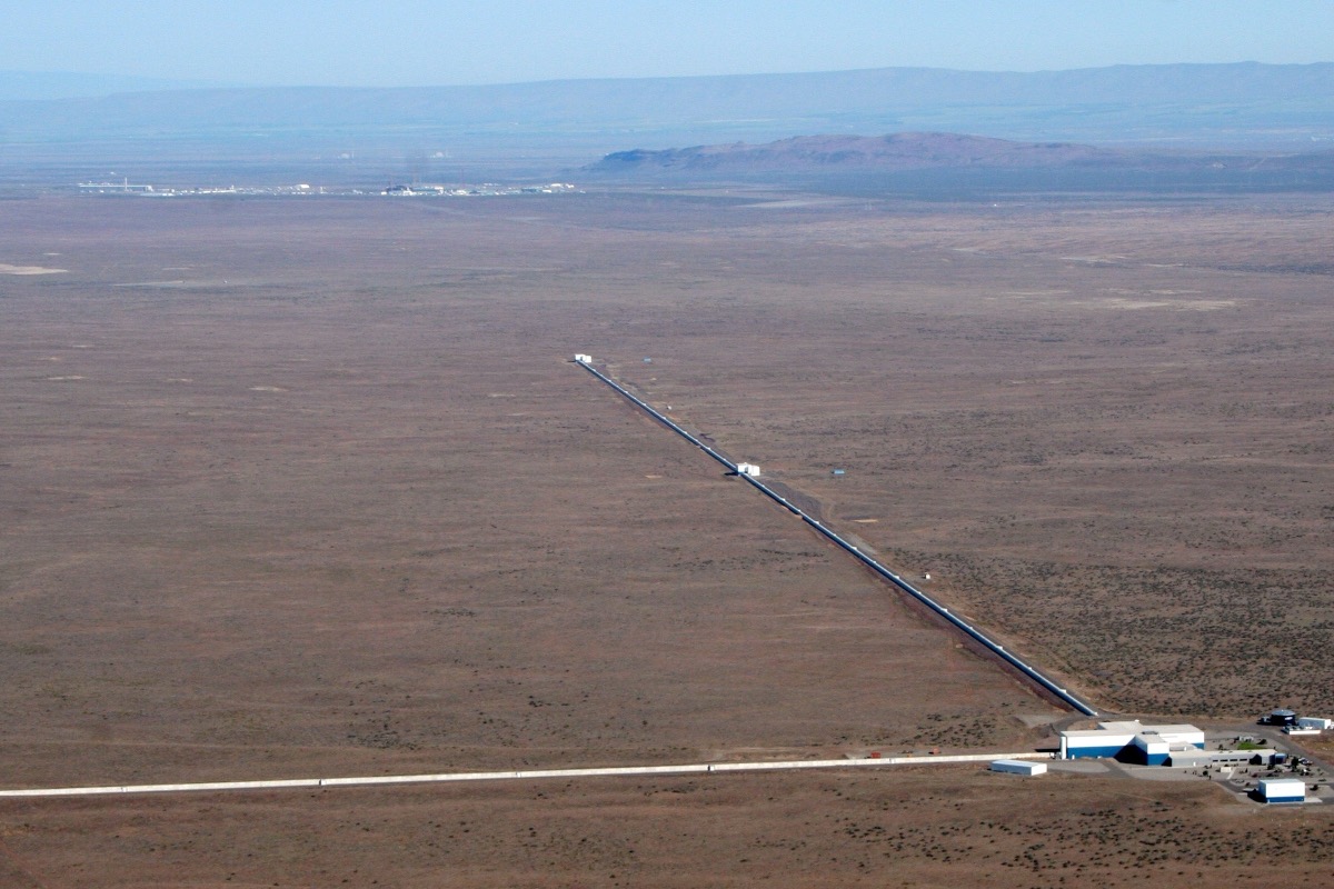
A gravitational-wave interferometer has thousands of coupled degrees of freedom — optical, mechanical, thermal, electronic — and its behavior changes hour to hour as alignment drifts, seismic conditions shift, and control loops interact. Commissioning a new detector (or recovering from a hardware change) requires painstaking manual diagnosis: measuring transfer functions, comparing them to models, identifying discrepancies, adjusting parameters, and repeating.

Digital twins — high-fidelity simulation models that shadow the real instrument in near-real time — can compress this process. Instead of waiting for the instrument to reveal its state through days of measurements, we interrogate the model: test hypotheses, train controllers, and predict failures in silico before touching the real machine.

---

Digital twins in practice

Origins and definition

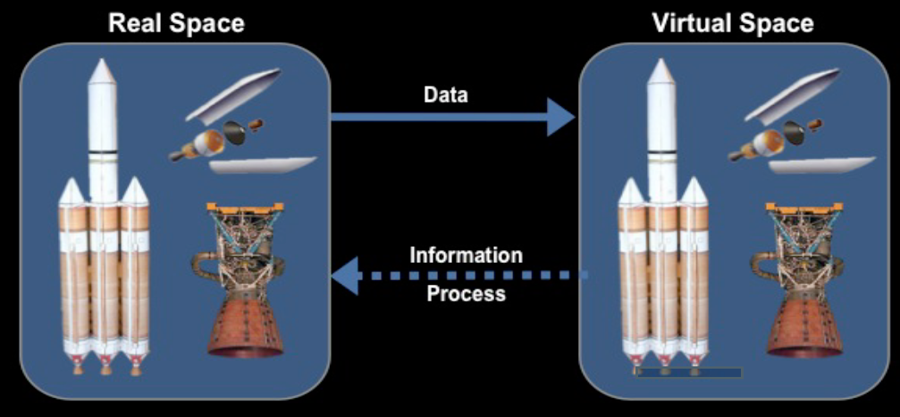
The term “digital twin” emerged from product lifecycle management. Michael Grieves introduced the concept in 2002–2003 at the University of Michigan, describing a virtual representation that mirrors a physical product throughout its life. Grieves formalized the idea in a 2014 white paper and, with John Vickers of NASA, in a 2017 Springer chapter (DOI 10.1007/978-3-319-38756-7_4). The canonical aerospace definition came from Glaessgen and Stargel at NASA in 2012 (AIAA 2012-1818): “an integrated multiphysics, multiscale, probabilistic simulation of an as-built vehicle or system that uses the best available physical models, sensor updates, fleet history, etc., to mirror the life of its corresponding flying twin.”

The key distinction from ordinary simulation: a digital twin tracks a specific individual system, updates continuously from sensor data, and evolves with the real system over its operational life. A flight simulator models an aircraft type; a digital twin models tail number N12345.

Aerospace: where the concept matured

The U.S. Air Force was an early adopter. Tuegel et al. (2011, International Journal of Aerospace Engineering) proposed per-tail-number structural life prediction for military aircraft, tracking fatigue crack growth in each individual airframe rather than relying on fleet-wide statistical models. The F-35 Joint Strike Fighter program implemented structural digital twins for every airframe, with Lockheed Martin reporting a 75% cost reduction in structural data products compared to traditional flight-test approaches.

The most rigorous mathematical framework came from Kapteyn, Pretorius & Willcox (2021, Nature Computational Science 1, 337), who formulated predictive digital twins as probabilistic graphical models — Bayesian networks that encode the relationships between model parameters, sensor observations, and predictions. They demonstrated the approach on a 12-foot-wingspan UAV, using real flight data to update structural models and predict remaining useful life. Ferrari & Willcox (2024, Nature Computational Science) reviewed how these ideas are reshaping mechanical and aerospace engineering more broadly.

Fusion energy: the closest analog to LIGO

Fusion reactors share LIGO’s core challenges: thousands of coupled degrees of freedom, plasma states that change on millisecond timescales, and experiments so expensive that simulation must substitute for trial and error. Morishita et al. (2024, Scientific Reports 14, 137) demonstrated the first digital-twin predictive control of a fusion plasma on the Large Helical Device (LHD) stellarator at NIFS, Japan — using real-time data assimilation to control electron temperature profiles via electron cyclotron heating.

Kates-Harbeck, Svyatkovskiy & Tang (2019, Nature 568, 526) showed that deep learning models trained on one tokamak (DIII-D) could predict disruptions on another (JET), demonstrating cross-machine transfer of learned physics — a direct analog to transferring a digital twin across detector sites. Most strikingly, Seo et al. (2024, Nature 626, 746) trained a reinforcement-learning controller in a tokamak simulation and deployed it on the real DIII-D machine to avoid tearing instabilities in real time. The parallel to the Deep Loop Shaping work — where RL controllers trained in SimPlant were deployed at LIGO Livingston — is immediate and direct.

Industrial fleets: gas turbines, jet engines, manufacturing

The largest operational digital twin deployments are in industrial asset management. Siemens’s ATOM platform maintains fleet-wide digital twins of gas turbines, tracking thermal creep, vibration spectra, and combustion dynamics to optimize maintenance scheduling across hundreds of units. GE Aviation operates digital twins for its jet engine fleet, reporting a 20% improvement in time-on-wing and significant reductions in unscheduled engine removals. These industrial twins demonstrate that the concept scales: the same framework applies whether you are tracking one system or thousands.

On the theoretical side, Qi & Tao (2018, IEEE Access 6, 3585) compared digital twin and big data approaches for smart manufacturing, while Rasheed, San & Kvamsdal (2020, IEEE Access 8, 21980) provided an influential review of digital twin modeling perspectives that has been cited over 900 times.

Particle accelerators and other big science

CERN’s Large Hadron Collider faces challenges remarkably similar to LIGO’s: a precision instrument with thousands of parameters, operating states that drift continuously, and experiments that cannot easily be interrupted for diagnostics. Arpaia et al. (2021, Nuclear Instruments and Methods A 985, 164652) demonstrated ML-augmented beam dynamics models for optics correction and beam loss prediction at the LHC. CERN’s interTwin project, through CERN openlab, is developing a general-purpose digital twin engine for large research infrastructures.

Nuclear power plants — where maintenance accounts for roughly 66% of operating expenditure — are also adopting the approach: Kropaczek et al. (2023, Springer) describe ORNL’s digital twin framework for reactor monitoring and predictive maintenance. The U.S. National Renewable Energy Laboratory’s ARIES platform applies similar ideas to power grid operations.

Common thread: why LIGO needs a digital twin

The pattern across all these domains is consistent. Systems that are too complex for manual diagnosis, have many coupled degrees of freedom, operate under constraints that make experimentation expensive or dangerous, and evolve over time — these are the systems where digital twins provide the most value. LIGO shares every one of these properties: thousands of coupled opto-mechanical degrees of freedom, an operating state that changes hourly, and experimentation that costs observing time during which real gravitational-wave events may be missed. The digital twin approach — a high-fidelity model continuously updated from sensor data — is the same across all domains. Only the physics engine changes.

Comparison of digital twins across domains

Domain	System	Coupled DOFs	Update rate	Key challenge
Aerospace	F-35 airframe	~10³ structural	Per flight	Fatigue crack growth
Fusion	Tokamak plasma	~10⁵ MHD modes	ms–s	Disruption avoidance
Gas turbine	SGT-A65	~10² thermal/mech	Minutes	Thermal creep
Particle accel.	LHC beam	~10⁴ optics params	Per fill	Beam loss
GW detector	LIGO DRFPMI	~10³ opto-mech	16 kHz–hours	Multi-scale coupling

EGG’s digital twin builds on SimPlant, a simulated interferometer plant framework developed at the Caltech 40m prototype since 2011. The current effort rebrands and expands SimPlant from a static simulation into a full digital twin with real-time state estimation, noise attribution, and calibration capabilities.

Contents:

• Digital twins in practice
• Prior work: SimPlant
• The simulation stack
• From SimPlant to digital twin
• State and parameter estimation
• Real-time noise budgets
• Physics-based calibration
• Pre-commissioning future detectors
• Technical challenges
• Prior work and publications
• Current status and future directions
• Key references

---

Prior work: SimPlant

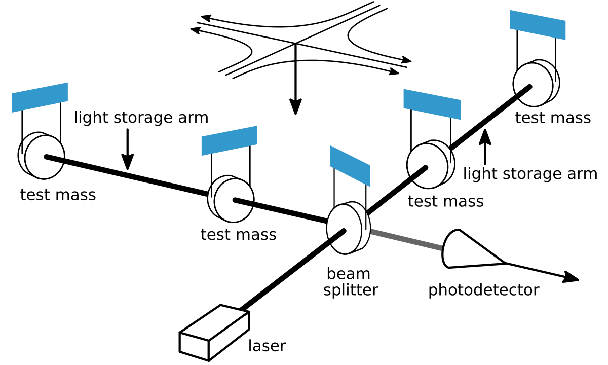
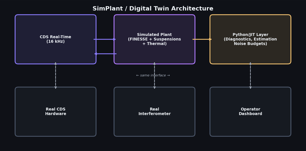
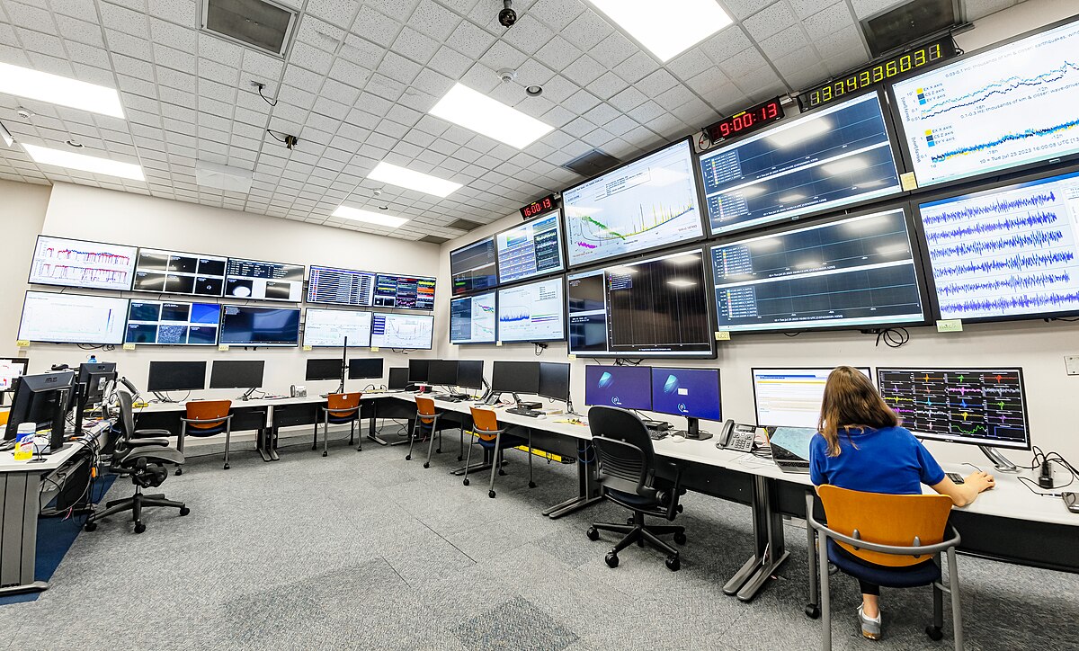
SimPlant is a simulated interferometer plant that runs on the same Control and Data System (CDS) infrastructure as the real detector. The key idea: the control code does not know — and does not care — whether it is talking to real mirrors or to a software simulation. Any controller tested in SimPlant is guaranteed to be compatible with the real hardware, because it runs through the identical digital signal processing chain.

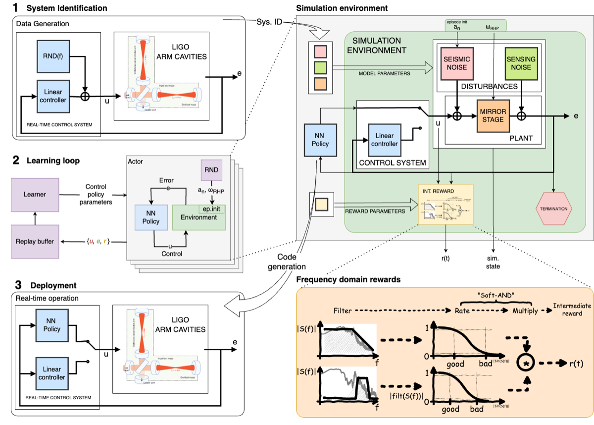
SimPlant was first demonstrated by Betzwieser in 2011 (LIGO-G1100524), initially developed at the Caltech 40m prototype. Arai, Rollins, Betzwieser & Adhikari expanded the framework in 2016 (LIGO-G1600511) with more complete optical, suspension, and servo models. SimPlant was subsequently used as the training environment for the Deep Loop Shaping reinforcement-learning controllers deployed at LIGO Livingston (Science 387, 540, 2025).

More recently, Chris Wipf developed RTSfreerun, a pure-Python CDS-like interface that allows anyone to run SimPlant-style simulations without access to the real CDS front-end hardware. RTSfreerun lowers the barrier to entry: a graduate student with a laptop can develop and test control configurations that are directly compatible with the production CDS environment.

---

The simulation stack

SimPlant assembles a complete interferometer simulation from specialized physics engines. No single tool handles all the physics — the simulation composes models across multiple domains.

Optical fields: FINESSE

FINESSE is the standard tool for modeling coupled optical cavities. It computes the steady-state and frequency-dependent response of the interferometer using a modal decomposition approach: each optical field is expanded in Hermite-Gaussian modes, and the interaction with each optical component (mirror, lens, beamsplitter) is described by scattering matrices. FINESSE solves for the self-consistent field amplitudes across the entire interferometer, including higher-order spatial modes, mirror figure errors, and radiation pressure effects.

For a cavity with mirrors of reflectivity $r_1, r_2$ and round-trip length $L$, the intracavity field buildup is:

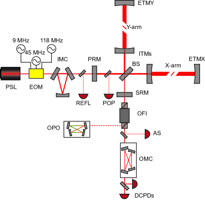
\[E_\text{circ} = \frac{t_1\, E_\text{in}}{1 - r_1\, r_2\, e^{i\,2kL}}\]

This simple expression becomes a system of coupled equations when the interferometer has dozens of mirrors, multiple coupled cavities, and feedback loops that modify the effective reflectivities. A single FINESSE simulation of the full LIGO dual-recycled Fabry-Perot Michelson interferometer (DRFPMI) takes on the order of seconds.

Mechanical suspensions

Multi-stage pendulum models (quadruple suspensions for test masses, triple suspensions for auxiliary optics) capture the measured mechanical transfer functions and cross-couplings. Seismic input is injected at the top stage using measured ground motion spectra. At frequencies below ~10 Hz, suspension dynamics dominate the interferometer response.

Thermal transients

Finite-element thermal models track mirror heating from laser absorption, ring heater actuation, and CO$_2$ laser compensation. Thermal lenses evolve on minutes-to-hours timescales, creating slow drifts that couple into alignment and mode-matching — the same physics modeled in the adaptive optics project.

Feedback electronics

All major servo loops (DARM, CARM, MICH, PRCL, SRCL, angular alignment, intensity stabilization) are modeled using the actual digital filter coefficients deployed at the sites, exported directly from the CDS configuration files.

Realistic noise injection

Seismic, thermal, shot, radiation pressure, and technical noise sources are injected with measured or modeled power spectral densities, producing synthetic data streams statistically consistent with real detector output. The result is simulation output in the same channel format as real detector data — a critical requirement for training and validating ML systems that must eventually process real data.

What are DARM, CARM, MICH, PRCL, SRCL?

LIGO’s control system manages multiple coupled degrees of freedom:

• DARM (Differential ARM): The gravitational-wave signal channel — the difference in arm lengths.
• CARM (Common ARM): The average arm length, kept on resonance with the laser.
• MICH (Michelson): The relative phase between the two arms at the beamsplitter.
• PRCL (Power Recycling Cavity Length): Controls the power recycling mirror position.
• SRCL (Signal Recycling Cavity Length): Controls the signal recycling mirror position.

Each degree of freedom has its own sensor (photodetector), actuator (electromagnetic coil on a suspension), and digital filter (servo loop). They interact through the optical fields: a change in PRCL affects the power in both arms, which changes DARM through radiation pressure. The digital twin must model all of these couplings simultaneously.

---

From SimPlant to digital twin

SimPlant as originally conceived is a static simulation: set the parameters, run the model, examine the output. A digital twin is a living model that tracks the real instrument continuously. The expansion from SimPlant to digital twin has two axes:

Runtime: SimPlant runs as an offline batch simulation. The digital twin operates in a hybrid real-time architecture:

• CDS real-time layer (16 kHz): The fast control loops (DARM, angular alignment, intensity stabilization) run on the same CDS front-end hardware as the real detector, at the same 16 kHz sample rate. This ensures exact compatibility between simulation and hardware.
• Python/JIT pseudo-real-time layer: Slower diagnostic computations — noise budgets, parameter estimation, thermal model updates — run in a Python environment with JIT compilation (Numba/JAX) at seconds-to-minutes cadence. This layer does not need to keep up with every sample, but must track the detector state on the timescale of its evolution.

Capabilities: The digital twin adds four new layers beyond SimPlant’s forward simulation:

1. State estimation — tracking the detector’s instantaneous configuration
2. Parameter estimation — keeping the underlying model synchronized with reality
3. Real-time noise budgets — continuous decomposition of detector noise
4. Physics-based calibration — model-driven supplement to the empirical calibration pipeline

---

State and parameter estimation

The detector’s state changes continuously. Mirror positions drift, alignment shifts, thermal lenses evolve, optical gain varies. A static simulation quickly goes stale. The digital twin must track all of this to remain useful.

State estimation (fast degrees of freedom)

Kalman-type filters infer the detector’s instantaneous state — mirror positions, angular misalignments, cavity mode content, thermal lens power — from the continuous stream of sensor data. The twin provides the system model: how the states evolve in time and how the sensors respond to each state variable. The filter optimally fuses the model’s predictions with noisy measurements, producing a running best-estimate of the detector configuration.

State estimation operates at the fast timescale (seconds or faster), tracking degrees of freedom that change on the timescale of control loop bandwidths.

Parameter estimation (slow drifts)

The underlying model parameters — cavity pole frequency, optical spring constant, suspension resonance frequencies, optical gain — drift over hours to days as the real detector evolves. Sources of drift include mirror contamination, electronics aging, alignment creep, and temperature variations. Parameter estimation tracks these slow changes, keeping the twin’s model synchronized with reality.

Unlike state estimation (which tracks where the detector is right now), parameter estimation tracks what the detector is — the slowly evolving physical properties that define its behavior.

Together

Fast state estimation tracks the detector’s instantaneous configuration. Slow parameter estimation keeps the underlying model accurate. Together, the twin never goes stale: it knows both where the detector is and what the detector has become.

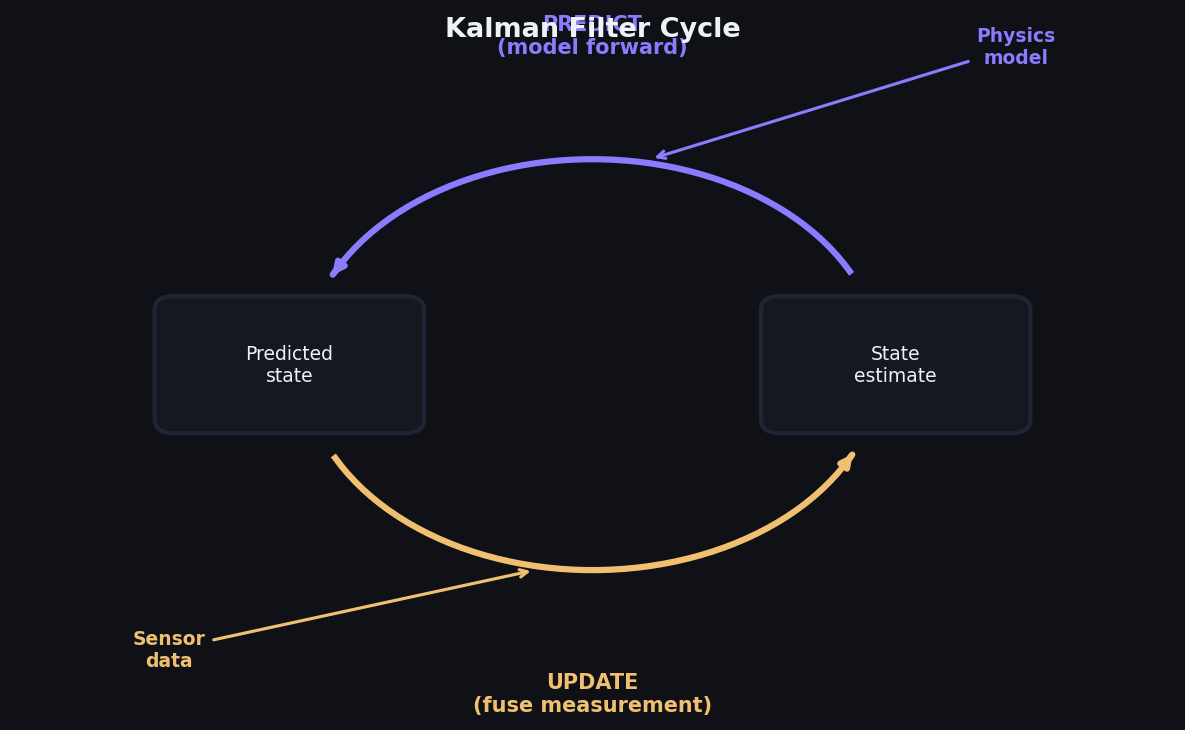
What is a Kalman filter?

A Kalman filter is an algorithm that estimates the state of a system from noisy measurements. It works in a two-step cycle:

1. Predict: Use the system model to predict what the state should be at the next time step, and how uncertain that prediction is.
2. Update: Compare the prediction to the actual measurement. If the measurement agrees with the prediction, trust the model. If it disagrees, adjust the state estimate toward the measurement, weighted by the relative uncertainties of model and measurement.

The filter is “optimal” in the sense that it minimizes the expected squared error when the system dynamics and noise are linear and Gaussian. For nonlinear systems like an interferometer, extended Kalman filters or ensemble methods provide approximate solutions.

The key insight is that the filter fuses two sources of information — the physics model and the measured data — in a principled way. A good model with noisy sensors still gives accurate state estimates, because the model constrains what states are physically plausible.

---

Real-time noise budgets

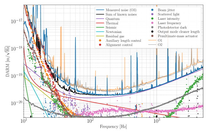
LIGO’s noise budget — the decomposition of total detector noise into individual physical sources — is currently computed offline, periodically, using tools like GWINC (Gravitational Wave Interferometer Noise Calculator). A digital twin can make this continuous.

Running theoretical budget

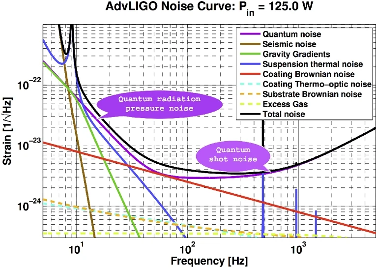
The twin continuously evaluates the theoretical noise floor: quantum shot noise, quantum radiation pressure noise, coating thermal noise, suspension thermal noise, seismic noise, and Newtonian gravity gradient noise, all computed using the twin’s current parameter estimates. As operating conditions change — laser power ramps up, squeezing level varies, alignment drifts — the noise budget updates in real time. This replaces periodic offline calculations with a live display that tracks the detector’s evolving noise floor.

Model-based noise decomposition

When measured noise exceeds the theoretical budget, the twin helps diagnose the source. By computing how each potential coupling path contributes to the gravitational-wave readout channel, the twin can attribute excess noise to specific mechanisms: electrical coupling at power-line harmonics, scattered light from a specific optical surface, mode mismatch at a cavity mirror, or acoustic coupling from a ventilation system.

Connection to neural network noise cleaning

The twin provides physics-informed priors for the neural network noise cleaning work: which auxiliary channels should couple to DARM, what the coupling transfer function should look like, and what frequency bands are most affected. The neural networks then learn the empirical residuals — the part of the coupling that the physics model does not fully capture. Together, physics model plus data-driven correction provides more robust noise subtraction than either approach alone.

What is GWINC?

GWINC (Gravitational Wave Interferometer Noise Calculator) is the standard tool for computing the fundamental and technical noise floors of a gravitational-wave detector. Given the detector’s design parameters — mirror masses, laser power, cavity lengths, coating properties, seismic spectra — GWINC evaluates each noise source as a function of frequency and produces the familiar “noise budget” plot showing which noise source limits sensitivity at each frequency.

Currently, GWINC is run offline with fixed parameters: an operator inputs the current detector configuration and gets a snapshot noise budget. The digital twin’s goal is to make this continuous — feeding GWINC-like calculations with live parameter estimates so the noise budget tracks the detector in real time.

---

Physics-based calibration

LIGO’s calibration pipeline converts raw photodetector signals into estimated gravitational-wave strain $h(t)$. This requires knowing the detector’s optomechanical response function — how a gravitational wave maps through the interferometer to the readout. The response function depends on the optical gain, cavity pole frequency, and actuation chain transfer functions, all of which vary with the detector’s operating state.

Currently, the response function is characterized by periodic swept-sine measurements and monitored using calibration lines (continuous sinusoidal excitations injected at known frequencies). Between calibration measurements, the response function is interpolated.

The twin’s role

The digital twin tracks the same physical parameters that determine the response function. Its continuously updated parameter estimates provide a running physics-based model of the optomechanical response, supplementing the empirical calibration pipeline. Where the empirical pipeline relies on periodic measurements, the twin provides continuous model-based estimates. Where the empirical pipeline interpolates between measurements, the twin fills in the gaps with physics.

Why this matters

Hall, Cahillane, Izumi, Smith & Adhikari (CQG 36, 205008, 2019) showed that systematic calibration errors propagate directly into biased astrophysical parameter estimates — affecting inferred masses, spins, and distances of detected gravitational-wave sources. The twin provides an independent, physics-based calibration channel that can catch errors the empirical pipeline might miss, or flag periods when the empirical and model-based calibrations disagree.

How LIGO calibration works

The calibration pipeline measures the detector’s response function — the transfer function from gravitational-wave strain to the DARM error signal — using two methods:

1. Photon calibrators: Auxiliary lasers that push on the test masses with known radiation pressure force. By measuring the resulting displacement, the actuation-to-displacement transfer function is characterized.
2. Calibration lines: Continuous sinusoidal excitations injected at specific frequencies. The measured response at these frequencies provides anchor points for the full response function.

The pipeline then deconvolves the measured response function from the DARM error signal to produce calibrated strain $h(t)$. The digital twin provides a model-based alternative: instead of relying on empirical measurements of the response function, the twin computes it from its current estimates of the physical parameters (optical gain, cavity pole, actuation strength). This model-based calibration can supplement the empirical pipeline, providing an independent cross-check and filling in between periodic measurements.

---

Pre-commissioning future detectors

One of the most powerful applications of the digital twin is building models of detectors that do not yet exist physically. By simulating the full instrument — optics, suspensions, controls, noise — before hardware is built, we can develop control systems, predict noise budgets, and identify design problems years before first light.

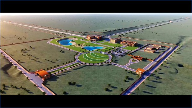
LIGO India

LIGO India, a third LIGO detector planned for Aundha Nagnath, Maharashtra, will use the same optical topology and CDS infrastructure as the existing LIGO detectors. A SimPlant model built from the as-designed instrument parameters could accelerate commissioning from first light by allowing control system development and testing years before the physical detector is complete. Controllers validated in the SimPlant twin would transfer directly to the real CDS hardware. See the LIGO India page for the broader context of the third detector.

A# and future detectors

LIGO’s next major upgrade (A#) will change the optical configuration: higher laser power, modified signal recycling, and new squeezing injection. The twin can predict how these design changes interact with the control system before hardware is procured. Questions that currently require building and testing — “Does this signal recycling configuration create new instabilities?” or “Can the angular control system handle the higher radiation pressure?” — can be explored in simulation first. The same approach extends to any future detector design: the digital twin becomes the first version of the instrument, the place where control systems are designed and noise budgets predicted before construction begins.

---

Technical challenges

Multi-scale temporal dynamics

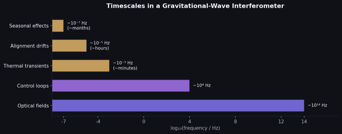
The interferometer spans more than 10 orders of magnitude in timescale: optical fields oscillate at $\sim 10^{14}$ Hz, control loops operate at $\sim 10^{4}$ Hz, thermal transients evolve over $\sim 10^{3}$ seconds, and seasonal drifts over $\sim 10^{7}$ seconds. No single model efficiently spans this range. The digital twin composes models operating at different timescales, passing information between them at appropriate rates.

Computational cost

The CDS real-time model must fit within 61 microseconds per cycle (the 16 kHz period). The Python/JIT diagnostic layer must keep up with data streams at seconds-scale latency. Both constraints demand reduced-order models and efficient numerical methods. Full-fidelity FINESSE simulations are too slow for either layer; the twin relies on pre-computed lookup tables, linearized models, and targeted high-fidelity checks.

Convergence of parameter estimation

The interferometer state space is high-dimensional. A naive Kalman filter tracking all physical parameters simultaneously is computationally intractable. Efficient approximate inference — ensemble methods, reduced-state estimators, hierarchical decomposition of fast and slow variables — is an active area of development.

Unmodeled physics

The real detector always has surprises: scattered light from unexpected surfaces, electronic interference at novel frequencies, noise sources that no one anticipated. The twin must gracefully handle regimes it was not built to model, flagging anomalies (large discrepancies between prediction and measurement) rather than producing silently wrong predictions.

System identification for interferometers

System identification — fitting model parameters to measured input-output data — is the bridge between the idealized twin and the real instrument. For LIGO, the standard approach is swept-sine transfer function measurement: inject a known excitation at each frequency and measure the response. This is accurate but slow — a full transfer function measurement of one control loop takes approximately 30 minutes.

Alternatives under investigation:

• Broadband excitation: Inject pseudo-random noise and use spectral estimation to recover the transfer function in a single measurement. Faster, but requires careful management of the excitation amplitude to avoid disturbing the interferometer’s operating point.

• Ambient identification: Use the naturally occurring noise (seismic, thermal) as the excitation and extract the transfer function from cross-spectral analysis. No injected excitation needed, but convergence is slow and biased by non-stationarity.

• Bayesian online estimation: Treat the model parameters as hidden states and use the continuous data stream to update posterior estimates. This is the “always-on” approach that would keep the twin synchronized with the real instrument, but requires efficient approximate inference algorithms to handle the dimensionality.

Each approach trades off measurement speed, accuracy, and invasiveness. The digital twin framework must support all of them, selecting the appropriate method based on the current operating state (commissioning vs. observing) and the parameters being estimated.

---

Prior work and publications

Prior work in this area from EGG includes:

• SimPlant framework — Betzwieser (2011, LIGO-G1100524); Arai, Rollins, Betzwieser & Adhikari (2016, LIGO-G1600511). CDS-compatible simulated interferometer plant.

• RL controller training — Buchli, Tracey, Andric, Wipf, Harms & Adhikari et al. (Science 387, 540, 2025; DOI). SimPlant served as the training environment for the Deep Loop Shaping controllers deployed at LIGO Livingston.

• Calibration error requirements — Hall, Cahillane, Izumi, Smith & Adhikari (CQG 36, 205008, 2019; DOI). Framework for understanding how systematic calibration errors propagate to astrophysical parameter biases.

---

Current status and future directions

What exists now:

• SimPlant is operational at the Caltech 40m prototype and has been used for RL controller training
• The basic simulation stack (FINESSE, suspension models, servo models, thermal models) is functional
• SimPlant’s CDS integration has been validated through the successful deployment of RL controllers at LIGO Livingston

In development:

• Expansion from static simulation to full digital twin with state and parameter estimation
• Real-time noise budget computation using the twin’s live parameter estimates
• Integration with the calibration pipeline as an independent physics-based cross-check
• Hybrid CDS/Python runtime architecture for the real-time and diagnostic layers

Future:

• Pre-commissioning models for LIGO India, A#, and future detectors
• Transfer of twin models across detector sites (Livingston, Hanford, India)
• Integration with neural network noise cleaning for combined physics-informed and data-driven diagnostics

Open questions:

• How much model fidelity is enough for each application (controller training, commissioning prediction, noise hunting)?
• How should the twin handle unmodeled physics — can anomaly detection be made reliable enough to flag problems without generating excessive false alarms?
• Can a twin developed for one detector site transfer to another with parameter adjustments, or do site-specific effects require building each twin from scratch?

---

Key references

SimPlant and digital twin development

• Betzwieser, “Real Controls with a Simulated Plant at the 40m,” LIGO-G1100524 (2011). DCC — First demonstration of SimPlant: real CDS control code driving a software model of the interferometer plant at the 40m prototype.

• Arai, Rollins, Betzwieser & Adhikari, “Simulated Plant Approach,” LIGO-G1600511 (2016). DCC — Expanded SimPlant framework with more complete optical, suspension, and servo models.

RL controllers trained in SimPlant

• Buchli, Tracey, Andric, Wipf, Harms & Adhikari et al., “Improving cosmological reach of a gravitational wave observatory using Deep Loop Shaping,” Science 387, 540 (2025). DOI — Demonstrated simulation-trained RL controllers transferring to real LIGO hardware, achieving significant noise reduction.

Calibration

• Hall, Cahillane, Izumi, Smith & Adhikari, “Systematic calibration error requirements for gravitational-wave detectors via the Cramér-Rao bound,” CQG 36, 205008 (2019). DOI — Framework for understanding how calibration systematics propagate to astrophysical parameter estimation biases.

Interferometer simulation tools

• Freise et al., “Interferometer simulation with FINESSE 3,” SoftwareX 17, 100916 (2022). DOI — The current version of the standard optical simulation tool for gravitational-wave interferometers.

LIGO detector performance

• Buikema et al., “Sensitivity and performance of the Advanced LIGO detectors in the third observing run,” PRD 102, 062003 (2020). DOI — Comprehensive description of the Advanced LIGO detector performance that the digital twin must reproduce.

• Staley et al., “Achieving resonance in the Advanced LIGO gravitational-wave interferometer,” CQG 31, 245010 (2014). DOI — Lock acquisition procedure that SimPlant must model for commissioning applications.

Digital twins across domains

• Grieves & Vickers, “Digital Twin: Mitigating Unpredictable, Undesirable Emergent Behavior in Complex Systems,” in Transdisciplinary Perspectives on Complex Systems, Springer (2017). DOI — Foundational chapter by the originator of the digital twin concept, formalizing the three-component model: physical entity, virtual entity, and data connections.

• Glaessgen & Stargel, “The Digital Twin Paradigm for Future NASA and U.S. Air Force Vehicles,” AIAA 2012-1818 (2012). DOI — Canonical definition of digital twins in aerospace: “integrated multiphysics, multiscale, probabilistic simulation of an as-built vehicle.”

• Kapteyn, Pretorius & Willcox, “A probabilistic graphical model foundation for monitoring-based digital twins,” Nature Computational Science 1, 337 (2021). DOI — Rigorous Bayesian framework for predictive digital twins, demonstrated on a UAV with real flight data.

• Kates-Harbeck, Svyatkovskiy & Tang, “Predicting disruptive instabilities in controlled fusion plasmas through deep learning,” Nature 568, 526 (2019). DOI — Deep learning disruption prediction on DIII-D and JET tokamaks, demonstrating cross-machine transfer of learned plasma physics.

• Morishita et al., “Digital twin of plasma for predictive control of fusion plasma,” Scientific Reports 14, 137 (2024). DOI — First demonstration of digital-twin predictive control of a fusion plasma, using real-time data assimilation on the LHD stellarator.

• Seo et al., “Avoiding satisficing in tokamak fusion plasmas,” Nature 626, 746 (2024). DOI — RL controller trained in simulation and deployed on real DIII-D hardware to avoid tearing instabilities — a direct parallel to the SimPlant/DLS approach.

• Rasheed, San & Kvamsdal, “Digital Twin: Values, Challenges and Enablers From a Modeling Perspective,” IEEE Access 8, 21980 (2020). DOI — Influential review (~930 citations) covering modeling frameworks, data-driven methods, and open challenges for digital twins across engineering domains.

• Arpaia et al., “Machine learning for beam dynamics studies at the CERN Large Hadron Collider,” Nuclear Instruments and Methods A 985, 164652 (2021). DOI — ML-augmented beam dynamics modeling for optics correction and beam loss prediction at the LHC.